Biology Driven Analyses of scRNA-Seq
Overview
Teaching: 120 min
Exercises: 10 minQuestions
What are some scRNA-Seq analyses that might provide me with biological insight?
Objectives
Gain an understanding of some of the important caveats for identifying major cell types in scRNA-Seq.
Understand the ability (and limitations) of scRNA-Seq data for quantifying differences in gene expression.
Have basic ability to be able to conduct enrichment analyses of gene expression in scRNA-Seq.
# set a seed for reproducibility in case any randomness used below
set.seed(1418)
Read Data from Previous Lesson
liver <- readRDS(file.path(data_dir, 'lesson05.rds'))
Batch correction
In bulk RNA-Seq experiments, it is usually vital that we apply a correction for samples profiled in different batches. In single cell RNA-Seq experiments the situation is a bit more nuanced. We certainly want to take into consideration if our samples have been profiled in different batches, but the point at which we do so can vary.
Consider this example. Distinguishing between cell types is a robust process, in fact we can do a fairly good job distinguishing major cell types with just a few dozen genes. We might expect that batch effects are small enough that they would not strongly impede our ability to identify cell types. We could do clustering and cell type identification, then when we are doing differential expression testing we could include a covariate for batch. This is an example where we would be appropriately considering batch, but not at every step in the analysis.
In contrast, in these liver data, we are going to show an example of why batch correction earlier in the analytical process can be helpful. The reason this section is included in the lesson on “biology-driven” analyses is that we will bring in some understanding of biology to show a specific example of cells that were separated (in UMAP space and in different clusters) by an unknown batch-related factor when they should have been clustering together as the same cell type.
We don’t know much about when these liver samples were profiled and what differences in the mice, equipment, or operators there could have been. There are 9 mice that were profiled in the data we are looking at. Let’s start by looking at whether specific cell clusters in our clustering + UMAP are derived largely from one or a few samples.
table(liver$sample, liver$seurat_clusters)
           0    1    2    3    4    5    6    7    8    9   10   11   12   13
  CS144   66   10    1   20    4  736    2 1747   77    8  990  135   35    0
  CS48     3    0   10    0   49    0 2028    2    0    0    0    7    0    0
  CS52     1    0    1    0 3815    0  941    0    1    5    0   46   86   24
  CS53     0    0    1 4284    4   21    8    0  650 1159    1    0    8  632
  CS88  3840  235 1154    0    8    4    1    1    5    0    0  206    4    0
  CS89   148  119  381    2    0  691    0    0  200    0    1   13  155    0
  CS92  3601  115  981    1    9    4    5    0    1    0    0  181    4    0
  CS96   299 4342 1965    0    0    3    1    0    4    0    0  312    3    0
  CS97    95  287  310   10    0 2321    1    0  575    1    3   20  434    0

          14   15   16   17   18   19   20   21   22
  CS144  274   74   51    0   33   87   31  162   12
  CS48     0    0    5    0    0   10    0    0    0
  CS52     0    0   35    0    0   71    0    1    8
  CS53     2    2    0  402  161    0   51    1    0
  CS88     0    0  123    0    0   39    2    0   24
  CS89   126  143    6    0   57    4   75   57    3
  CS92     0    0  105    0    0   36    1    0   17
  CS96     0    0  198    0    1   73    2    0   37
  CS97   246  330    9    0  141    7  153   90    1
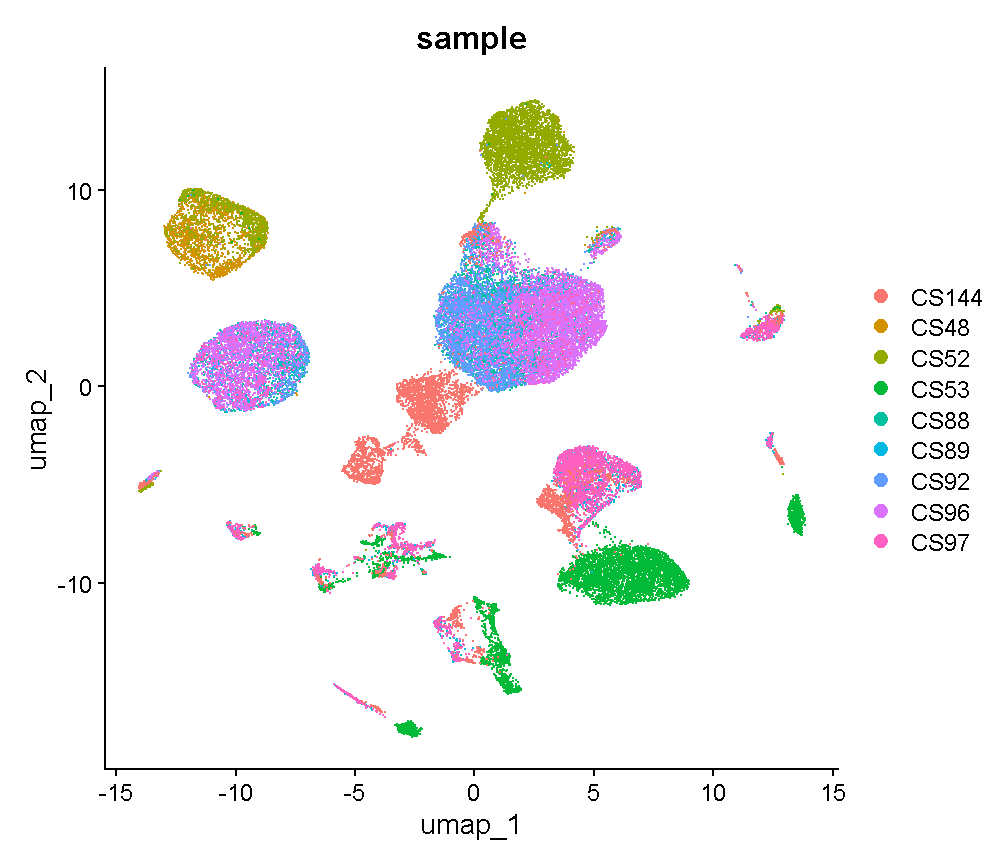
Notice cluster 13. Most of the cells are derived from mouse CS53. Let’s look into this a little further. First we plot the cells in UMAP space colored by mouse of origin, demonstrating some fairly clear batch effects – indicated by
- cell clusters that contain dots of only one or a few colors
- clusters of different colors that are near each other but not overlapping
UMAPPlot(liver, group.by = 'sample', pt.size = 0.1)
plot of chunk sample_effects
Let’s see which genes are expressed in cluster 13.
markers13 <- FindMarkers(liver, '13', only.pos = TRUE, logfc.threshold = 1,
                         max.cells.per.ident = 500)
head(markers13, 6)
              p_val avg_log2FC pct.1 pct.2     p_val_adj
Cd79a 1.522138e-182   7.370387 0.998 0.011 3.062541e-178
Ighm  9.697775e-180   5.805552 0.998 0.088 1.951192e-175
Cd79b 4.198563e-177   6.551524 0.989 0.060 8.447508e-173
Ebf1  2.315879e-175   7.085958 0.968 0.010 4.659549e-171
Igkc  1.606549e-172   7.293541 0.974 0.058 3.232376e-168
Iglc2 3.423234e-164   6.956922 0.939 0.015 6.887546e-160
We’ll talk in detail about the information in this type of table later. For now, just be aware that these are genes that are expressed much more highly in cluster 13 than in the other cells.
Look at the genes we are finding. These genes are expressed in almost
all cells of cluster 13 (column pct.1) and in few of the cells in other
clusters (column pct.2).
An immunologist would likely recognize these as B cell genes. The gene
Cd79a is very frequently captured well in single cell transcriptomics and
is highly specific to B cells. Let’s look at where Cd79a is expressed.
VlnPlot(liver, 'Cd79a')
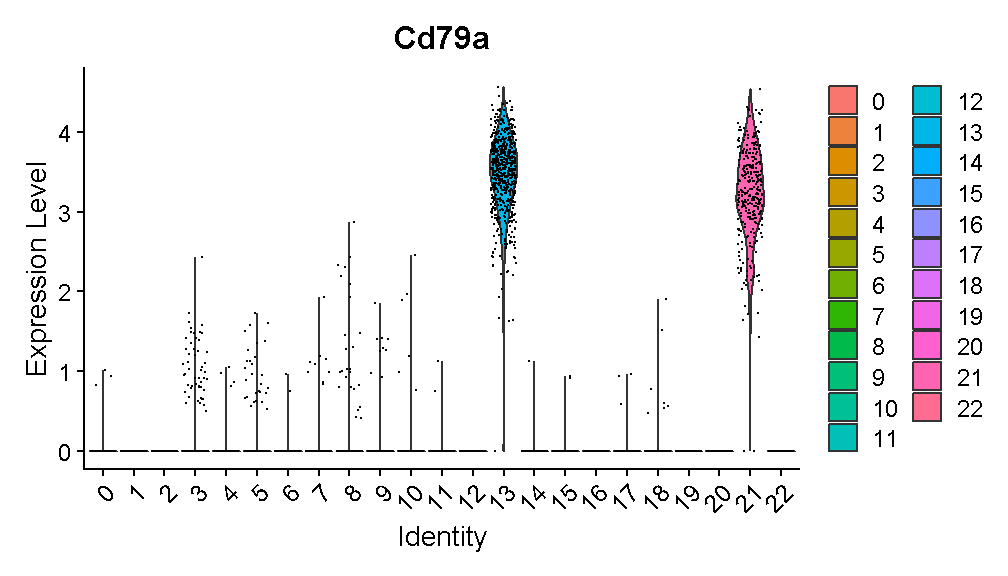
plot of chunk cd79a_vln
Expression of this gene is very clearly ON in clusters 13 and 21, and OFF in all other clusters. Let’s look at where clusters 13 and 21 are:
FeaturePlot(liver, "Cd79a", cols = c('lightgrey', 'red'),
            label = TRUE, label.size = 6)
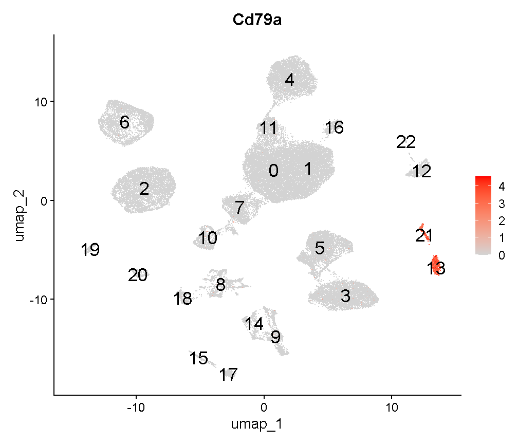
plot of chunk cd79a_fp
Interesting. Clusters 13 and 21 are near each other. Recall that we saw that cluster 13 cells are largely derived from a single mouse. Looking at cluster 21:
table(liver$sample[liver$seurat_clusters == '21'])
CS144  CS52  CS53  CS89  CS97
  162     1     1    57    90
we can see that this cluster contains cells from several mice. Both clusters 13 and 21 are B cells – you can verify this on your own by looking at expression of other B cell marker genes. It is unlikely that there would be heterogeneous types of B cells that segregate almost perfectly between different batches. Rather, it seems that there is some batch-driven pattern in gene expression that is causing these cells to cluster separately when they should cluster together.
In the liver cell atlas paper Guilliams et al from which we obtained these data, the authors applied a batch correction across samples. They used a method called harmony. We will run harmony on the subset of data that we are working with. We expect that a successful batch correction algorithm will bring the cells in clusters 13 and 21 together into a single cluster.
Harmony is an algorithm that projects cells into a shared low-dimensional embedding. In an iterative process, harmony learns cell-specific linear adjustment factors in order to integrate datasets in a way that favors clusters containing cells from multiple datasets. At the same time, the method has features that allow it to maintain separation of cell clusters that are unique to particular datasets. The harmony method is described in Korsunsky et al. 2019 and has a website at this link. The following animation, available from this link in a beautiful and comprehensive workup by Kamil Slowikowski, shows in a visual manner how cells from different donors are integrated together
Let’s run harmony on the liver data. Harmony itself returns a low-dimensional embedding of the cells, much like the reduced dimensional embedding of cells that we previously produced in PC-space. Recall that we performed clustering and projection to two dimensions with UMAP all using the PCA dimension reduction. We will now redo those steps but use the harmony reduction instead. Note that harmony has several parameters that could be tweaked. The most important may be theta. Higher values of theta force more mixing across batches. We will use the same values of each parameter that the authors of the liver cell atlas used – their code is available at this link.
After we run harmony using the same parameters the authors used, we will look at the harmony components and decide how many to use – in a way analogous to deciding how many PCs to use for UMAP and clustering.
# Store old UMAP and old clusters
liver$before_harmony_clusters <- liver$seurat_clusters
liver@misc$noharmony_umap <- liver@reductions$umap

# Run harmony
liver <- RunHarmony(liver, 'sample', assay.use='RNA',
           theta=1, dims.use=1:40, max.iter.harmony=100)
ElbowPlot(liver, reduction = 'harmony', ndims = 40)
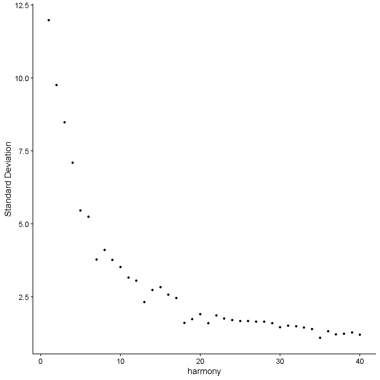
plot of chunk harmony
Let’s again pick 24 dimensions, just like we looked at 24 dimensions in PC space.
liver <- FindNeighbors(liver, reduction = 'harmony', dims = 1:24) %>%
         FindClusters(verbose = FALSE, resolution = 0.3) %>%
         RunUMAP(dims = 1:24, reduction = 'harmony')
Computing nearest neighbor graph
Computing SNN
02:26:05 UMAP embedding parameters a = 0.9922 b = 1.112
02:26:05 Read 44253 rows and found 24 numeric columns
02:26:05 Using Annoy for neighbor search, n_neighbors = 30
02:26:05 Building Annoy index with metric = cosine, n_trees = 50
0% 10 20 30 40 50 60 70 80 90 100%
[----|----|----|----|----|----|----|----|----|----|
**************************************************|
02:26:09 Writing NN index file to temp file C:\Users\c-dgatti\AppData\Local\Temp\Rtmpua4Qd7\file2e34780d10a1
02:26:09 Searching Annoy index using 1 thread, search_k = 3000
02:26:20 Annoy recall = 100%
02:26:21 Commencing smooth kNN distance calibration using 1 thread with target n_neighbors = 30
02:26:24 Initializing from normalized Laplacian + noise (using RSpectra)
02:26:34 Commencing optimization for 200 epochs, with 1888044 positive edges
02:27:12 Optimization finished
liver$after_harmony_clusters <- liver$seurat_clusters
Now let’s see where the cells from the former clusters 13 and 21 appear in our new clustering.
table(liver$before_harmony_clusters,
      liver$after_harmony_clusters)[c('13', '21'), ]
       0   1   2   3   4   5   6   7   8   9  10  11  12  13  14  15
  13   0   0   0   0   0   0   0 656   0   0   0   0   0   0   0   0
  21   0   0   0   1   0   0   0 310   0   0   0   0   0   0   0   0
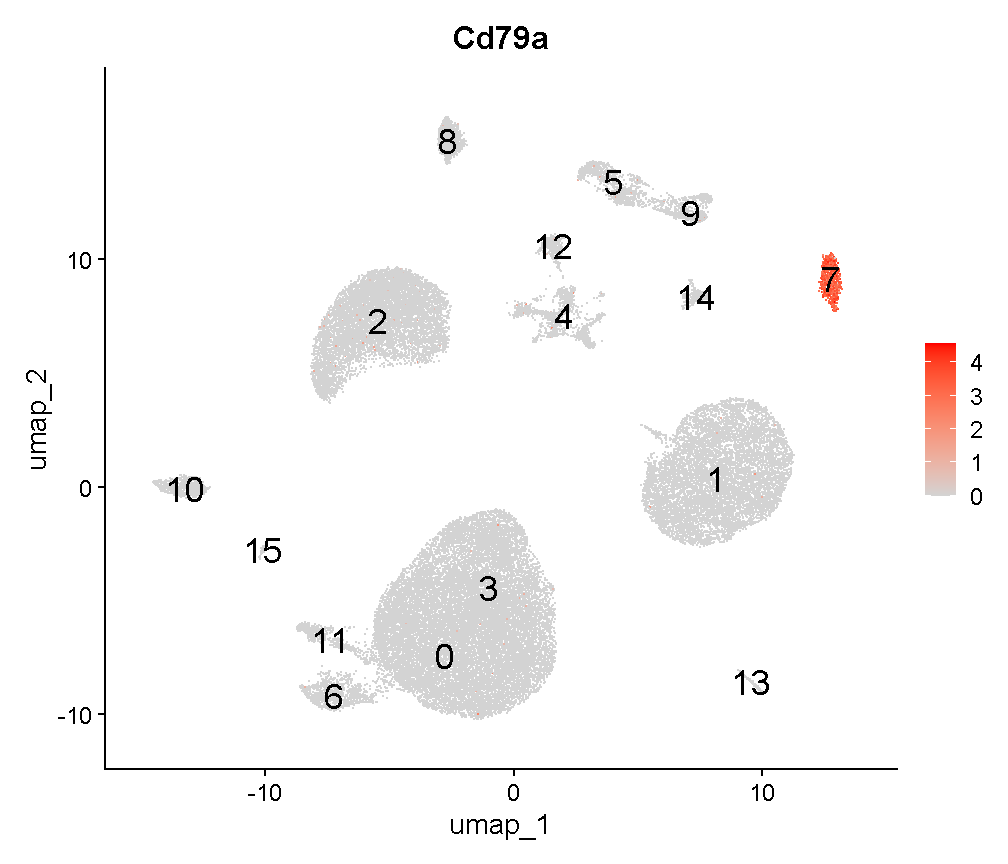
These cells are nearly all in one new cluster. This cluster exclusively expresses the B cell gene Cd79a, suggesting that the harmony batch correction has accomplished the task that we had hoped.
FeaturePlot(liver, 'Cd79a', cols = c('lightgrey', 'red'), label = T,
            label.size = 6)
plot of chunk c8
VlnPlot(liver, 'Cd79a')
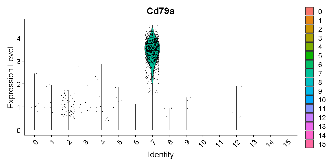
plot of chunk c9
We will work with the harmony clusters from this point forward. In a real analysis we should spend more time trying different parameters and verifying that our results are robust to a variety of different choices. We might also examine other cell clusters that were specific to one batch in an effort to determine whether they are like this B cell example and should be better aligned between batches, or whether the cells are truly unique to that batch and should not be aligned with cells present in other batches.
Next we take a step specific to this lesson that would not normally be a part of your single cell data analysis. While developing the course content we found some variability in the numbers assigned to clusters. This may be due to minor variations in package versions, because we do set a seed for random number reproducibility. In the next chunk we rename clusters to ensure that we are all working with a common cluster numbering system. Don’t worry about how we got this list of genes for now.
genes <- c('Socs3', 'Gnmt', 'Timd4', 'Ms4a4b', 'S100a4',
           'Adgrg6', 'Cd79a', 'Dck', 'Siglech', 'Dcn',
           'Wdfy4', 'Vwf', 'Spp1', 'Hdc')
Idents(liver) <- 'after_harmony_clusters'
a <- AverageExpression(liver, features = genes)[['RNA']]
As of Seurat v5, we recommend using AggregateExpression to perform pseudo-bulk analysis.
First group.by variable `ident` starts with a number, appending `g` to ensure valid variable names
This message is displayed once per session.
highest_clu <- unname(colnames(a))[apply(a, 1, which.max)]

cluster_converter <- setNames(paste0('c', c(0:1, 3:14)), highest_clu)
remaining_clusters <- setdiff(as.character(unique(Idents(liver))),
                              highest_clu)
a <- AverageExpression(subset(liver, idents = remaining_clusters),
                       features = c("Lyve1", "Cd5l"))[['RNA']]
highest_clu <- unname(colnames(a))[apply(a, 1, which.max)]
cluster_converter[highest_clu] <- c('c2', 'c15')

liver$renamed_clusters <- cluster_converter[as.character(liver$after_harmony_clusters)]
Error in if (length(x = value) == ncol(x = x) && all(names(x = value) == : missing value where TRUE/FALSE needed
Idents(liver) <- 'renamed_clusters'
Finding marker genes
Now we will find marker genes for our clusters. Finding marker genes takes a
while so we will downsample our data to speed up the process.
The downsample argument to the subset() function means that Seurat
will take a random 300 (maximum) cells from each cluster in our
liver_mini object.
Even with the downsampled data this marker-finding will take a few minutes.
liver_mini <- subset(liver, downsample = 300)
markers <- FindAllMarkers(liver_mini, only.pos = TRUE,
                          logfc.threshold	= log2(1.25), min.pct = 0.2)
Warning: No DE genes identified
Warning: The following tests were not performed:
Warning: When testing renamed_clusters versus all:
	Cells in one or both identity groups are not present in the data requested
These cluster marker genes are very useful. By definition, the marker genes vary in expression between the cells in our dataset. Therefore each gene is helping to capture some aspect of the cellular heterogeneity found within the liver tissue we profiled.
The most important task we will carry out using our marker genes is
the identification of cell type labels for each cluster.
One approach to obtaining cell type labels is to use an automated
method like SingleR, which was introduced in
Aran et al. 2019
and has a companion Bioconductor package
here.
This method
performs unbiased cell type recognition from single-cell RNA sequencing data, by leveraging reference transcriptomic datasets of pure cell types to infer the cell of origin of each single cell independently.
A method like SingleR is a great option for taking a first look at your
data and getting a sanity check for what cell types are present.
However, we find that the reference cell type data are often insufficient
to categorize the full cellular diversity in many datasets.
An automated method might be a great way to initially identify
T cells, macrophages, or fibroblasts – but might struggle with
categorizing more detailed subsets like inflammatory macrophages or
activated fibroblasts.
The “classic” way to identify cell types in your scRNA-Seq data is by looking at the marker genes and manually labelling each cell type. This manual method has been used ever since the first single cell transcriptomic studies of tissue cellular heterogeneity. There are both advantages and disadvantages to the manual approach. The advantages include:
- The ability to utilize considerable subjective judgement – after all, you should be familiar with the tissue you are looking at and you can label cells with arbitrary levels of precision and descriptiveness
- The possibility to identify cells that are not well represented in
existing data/databases like that used by
SingleR
Disadvantages include:
- This method can be slow and tedious;
- Your biological knowledge of the tissue might cause you to mislabel cells.
We will show an example of this type of cell type identification below.
One could also integrate your data with other existing datasets that have cell labels, and do label transfer. There is more information on this topic in lesson 7 where you will have the opportunity to (potentially) try out this approach on your own data. This is a very useful approach that is likely to become increasingly useful as the scientific community accumulates more and more scRNA-Seq datasets.
Identifying cell types
Let’s plot the expression of some of the major cell type markers. Look at the
data.frame markers for a summary of the markers we found above. We’ll massage
the markers data.frame into a more tidy format:
old_markers <- markers
markers <- as_tibble(markers) %>%
              select(cluster, gene, avg_log2FC, pct.1, pct.2, p_val_adj)
Error in `select()`:
! Can't select columns that don't exist.
✖ Column `cluster` doesn't exist.
head(markers, 6)
data frame with 0 columns and 0 rows
In the markers tibble, the columns have the following meanings:
- cluster – the cluster in which expression of the marker gene is enriched
- gene – the gene that has high expression in this cluster
- avg_log2FC – the log2 fold change difference in expression of the gene between this cluster compared to all the rest of the cells
- pct.1 – the fraction of cells in this cluster that express the gene (expression is just quantified as a nonzero count for this gene)
- pct.2 – the fraction of cells not in this cluster (i.e. all other cells) that express the gene
- p_val_adj – a multiple testing corrected p-value (Bonferroni corrected) for the marker indicating the significance of expression enrichment in this cluster compared to all other cells
You should be aware of one weakness of finding cell types using this approach. As mentioned above, this marker gene-finding function compares expression of a gene in cluster X to expression of the gene in all other cells. But what if a gene is highly expressed in cluster X and in some other tiny cluster, cluster Y? If we compare cluster X to all other cells, it will look like the gene is specific to cluster X, when really the gene is specific to both clusters X and Y. One could modify the marker gene-finding function to compare all clusters in a pairwise fashion and then unify the results in order to get around this issue. Dan Skelly has some code available here that implements such an approach in the Seurat framework, should you wish to try it.
In this course, we will not get into this level of detail.
Let’s look at the top 3 markers for each cluster:
group_by(markers, cluster) %>%
  top_n(3, avg_log2FC) %>%
  mutate(rank = 1:n()) %>%
  pivot_wider(id_cols = -c(avg_log2FC, pct.1, pct.2, p_val_adj),
              names_from = 'rank', values_from = 'gene') %>%
  arrange(cluster)
Error in `group_by()`:
! Must group by variables found in `.data`.
✖ Column `cluster` is not found.
Recognizing these genes might be a big challenge if you are not used to looking at single cell gene expression. Let’s check out expression of the very top genes in each cell cluster:
top_markers <- group_by(markers, cluster) %>%
                 arrange(desc(avg_log2FC)) %>%
                 top_n(1, avg_log2FC) %>% pull(gene)
Error in `group_by()`:
! Must group by variables found in `.data`.
✖ Column `cluster` is not found.
VlnPlot(liver, features = top_markers, stack = TRUE, flip = TRUE)
Error: object 'top_markers' not found
What does this tell us? Well, there are some genes here that are quite specific to one cluster (e.g. S100a9, Spp1, Ccl5, Siglech), but there are a few markers that are not very good markers at all (e.g. Fabp1, Cst3) and some that are not very specific (e.g. Clec4f, Cd5l, Kdr, Clec4g).
Let’s look at one of these last kinds of markers – Kdr. Our violin plot above shows that this gene is expressed in clusters c0, c6, c12, and c2. If we look at a UMAP plot
UMAPPlot(liver, label = TRUE, label.size = 6) + NoLegend()
plot of chunk expr
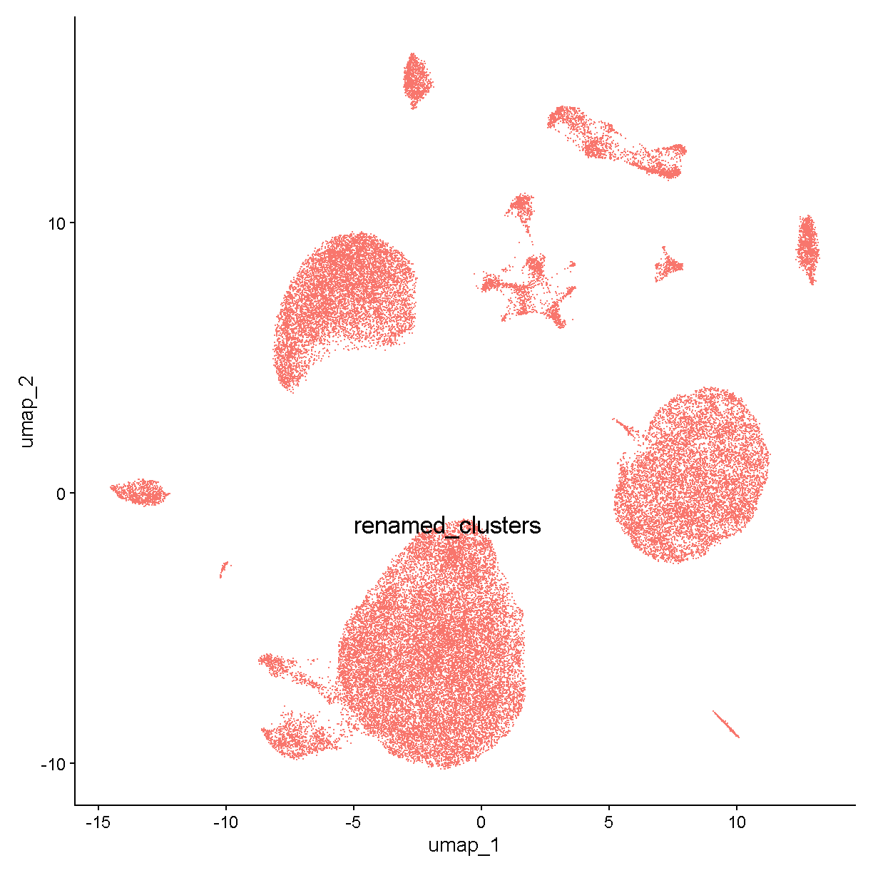
we see that these clusters are smaller bits of a large cloud of points in UMAP space. This is probably a relatively heterogenous cell type or or a continuum of cells (e.g. differentiating cells or cells being activated by some stimulus). Nevertheless it is fairly clear that these cells all express Kdr:
FeaturePlot(liver, features = "Kdr", cols = c('lightgrey', 'red'))
plot of chunk expr2
If we do some digging, we see that Kdr encodes vascular endothelial growth factor receptor 2. In the liver, we would expect endothelial cells to be fairly abundant. Therefore we can already say with relatively high confidence that clusters c0, c2, c6, and c12 are endothelial cells.
Looking again at the violin plot above, there are some genes that are often seen in scRNA-Seq data and are excellent markers:
- S100a9 is a marker for neutrophils (or the broader category of granulocytes) - c14
- Ccl5 (which encodes RANTES) is a marker for T cells. The T cell cluster might also include some other related immune cell types (natural killer [NK] cells and innate lymphoid cells [ILCs]) - c4
- Siglech is a marker for plasmacytoid dendritic cells - c9
We have now identified (at least tentative) cell types for clusters c0, c2, c4, c6, c9, c12, and c14.
Let’s turn to those markers that seemed to be expressed across all or almost all cell types (recall Cst3 and Fabp1). Let’s focus on cluster c1. This is a pretty large cluster. In our violin plot cluster c1 is marked only by Fabp1, which is much higher in cluster c1 than in any other cluster, but still has high background in ALL clusters.
Doing a bit of sleuthing, we find that Fabp1 is expressed in hepatocytes. For example, this reference says that Fabp1 is found abundantly in the cytoplasm of hepatocytes. It also makes sense that cluster c1 is hepatocytes because this cluster is large and we expect a lot of hepatocytes in the liver.
However, why do we see high background levels of Fabp1? The reason might be due to ambient RNA. If a liver cell lyses and releases its contents into the “soup”, the cell’s RNA molecules could tag along for the ride in any droplet with any other cell type. This ambient RNA would act as noise in the transcriptome of each cell. The problem of ambient RNA can vary considerably between samples. A recent paper by Caglayan et al gives a nice case study and examines the phenomenology of ambient RNA in single nucleus RNA-Seq. There are several methods to correct for high levels of ambient RNA, with CellBender showing good performance in multiple studies. We will not apply an ambient RNA correction for this course.
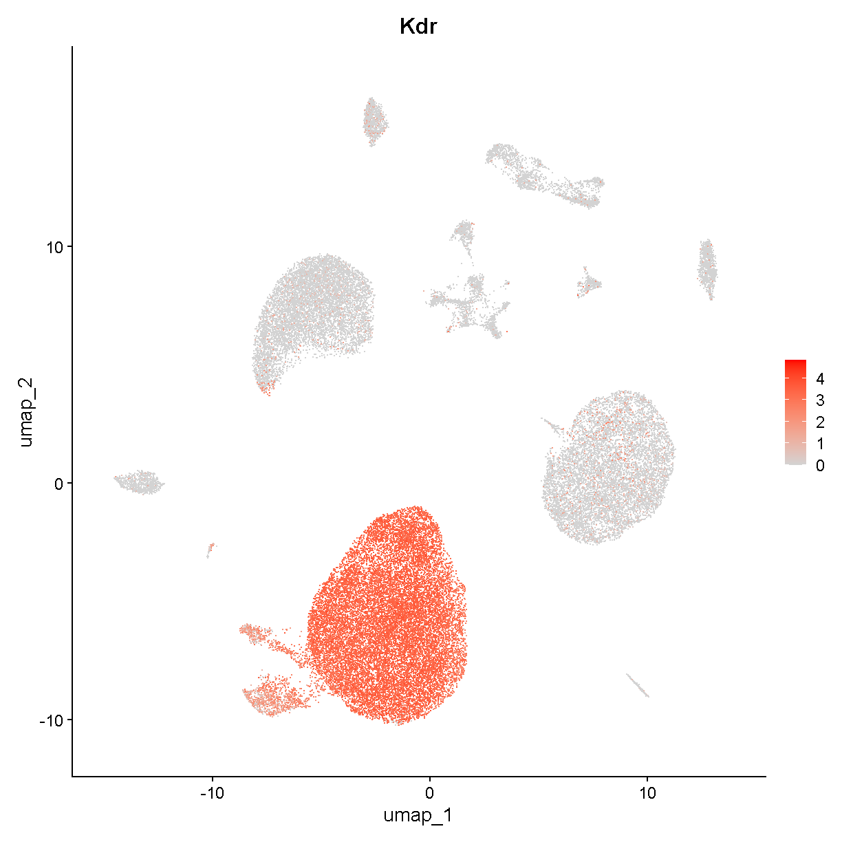
To examine whether these data show evidence of a hepatocyte ambient RNA signature, we start by looking at our non-specific marker Fabp1:
FeaturePlot(liver, "Fabp1", cols = c('lightgrey', 'red'),
            label = TRUE, label.size = 6)
plot of chunk expr3
This seems consistent with our expectations based on what we know about ambient RNA. Let’s look at another hepatocyte marker:
FeaturePlot(liver, "Serpina1a", cols = c('lightgrey', 'red'),
            label = TRUE, label.size = 6)
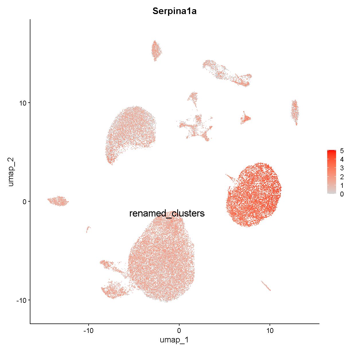
plot of chunk expr4
Very similar. We tentatively conclude that this dataset has a noticeable amount of hepatocyte ambient RNA contributing to all cell transcriptomes. Let’s label cluster c1 as hepatocytes.
Because of Fabp1 and other noisy markers in our cluster-specific gene expression data.frame, we’ll try filtering our markers to grab only those that are not expressed too highly (on average) in all the other cells:
specific_markers <- group_by(markers, cluster) %>%
  arrange(desc(avg_log2FC)) %>%
  filter(pct.2 < 0.2) %>%
  arrange(cluster) %>%
  top_n(1, avg_log2FC) %>% pull(gene)
Error in `group_by()`:
! Must group by variables found in `.data`.
✖ Column `cluster` is not found.
VlnPlot(liver, features = specific_markers, stack = TRUE, flip = TRUE)
Error: object 'specific_markers' not found
This looks better – the markers are more specific. We do have a marker for the hepatocytes (cluster c1) that looks better than before. However, this gene – Inmt – does not seem to be a very good hepatocyte marker according to the literature. Thus our filter to remove non-specific markers may have gotten rid of most of the strongly hepatocyte-specific gene expression.
In this violin plot we do have some instances where a marker seems to be specific to two or three cell clusters (e.g. Vsig4, Stab2, etc).
Stab2 is marking the endothelial cells we already identified (or at least some of them). Let’s look at Vsig4:
FeaturePlot(liver, "Vsig4", cols = c('lightgrey', 'red'), label = TRUE,
            label.size = 6)
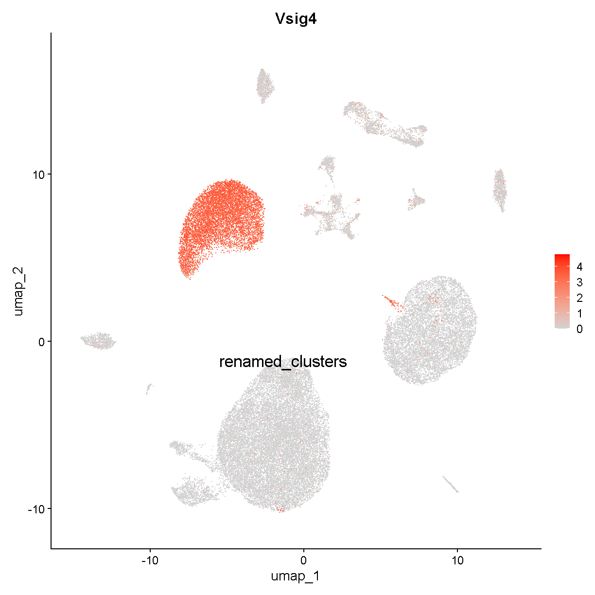
plot of chunk vsig4
This is marking clusters c3, c8, and c15. Clusters c3 and c8 are very near each other. Vsig4 is an immune protein (V-set and immunoglobulin domain containing 4). The protein is expressed selectively in – among other cell types – Kupffer cells, which are the resident macrophages in the liver. Clusters c3 and c8 may be Kupffer cells. Let’s check a famous macrophage marker, F4/80 (gene name Adgre1):
FeaturePlot(liver, "Adgre1", cols = c('lightgrey', 'red'), label = TRUE,
            label.size = 6)
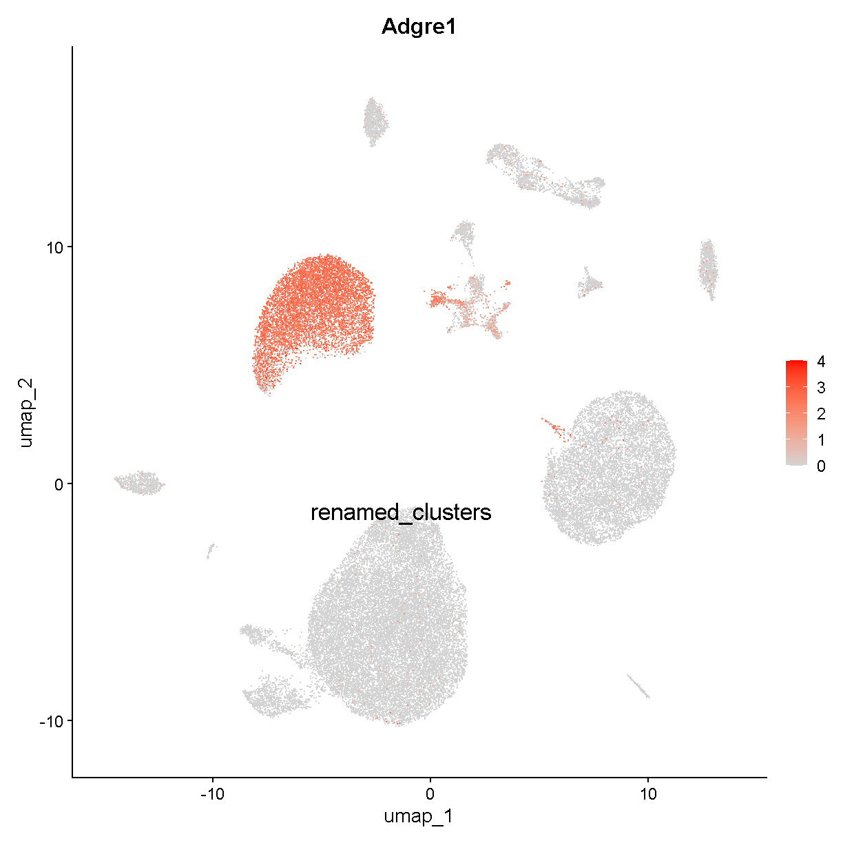
plot of chunk adgre1
Cluster c15 expresses Adgre1 but is near the hepatocyte cluster we just discussed. In fact it is located between the hepatocyte and Kupffer cell clusters. Cluster c15 might represent hepatocyte-Kupffer cell doublets. Consistent with this theory, cluster c15 has intermediate expression of Kupffer cell-specific Adgre1 and hepatocyte-specific Fabp1.
VlnPlot(liver, c("Adgre1", "Fabp1"), idents = c('c3', 'c15', 'c1'), sort = T)
Error in `FetchData()`:
! None of the cells requested found in this assay
Let’s store our labels and look at what remains unidentified.
labels <- tibble(cluster_num = unique(liver$renamed_clusters)) %>%
          mutate(cluster_num = as.character(cluster_num)) %>%
          mutate(cluster_name = case_when(
                 cluster_num %in% c('c0', 'c2', 'c6', 'c12') ~ 'ECs',   # endothelial cells
                 cluster_num == 'c1' ~ 'hepatocytes',
                 cluster_num %in% c('c3', 'c8') ~ 'Kupffer cells',
                 cluster_num == 'c4'  ~ 'T cells',
                 cluster_num == 'c7'  ~ 'B cells',
                 cluster_num == 'c9'  ~ 'pDCs',               # plasmacytoid dendritic cells
                 cluster_num == 'c14' ~ 'neutrophils',
                 cluster_num == 'c15' ~ 'KH doub.',          # Kupffer-hepatocyte doublets
                 TRUE ~ cluster_num))
Error in (function (cond) : error in evaluating the argument 'x' in selecting a method for function 'unique': 'renamed_clusters' not found in this Seurat object
 Did you mean "seurat_clusters"?
liver$labels <- deframe(labels)[as.character(liver$renamed_clusters)]
Error in x[[1]]: object of type 'closure' is not subsettable
UMAPPlot(liver, label = TRUE, label.size = 6, group.by = 'labels') + NoLegend()
Warning: The following requested variables were not found: labels
Error in `[.data.frame`(data, , group): undefined columns selected
Challenge 1
We have identified the cell types for several large clusters. But there are still several unlabelled clusters. We will divide the class into groups, each of which will determine the cell type for one of the remaining clusters. How should you do this? If you have a background in liver it may be as simple as looking for genes you recognize as being involved in the tissue’s biology. More likely you are not a liver expert. Try doing a simple Google search. You could Google “gene cell type” or “liver gene”. Look at the results and see if you get any clues to the cell type. This might include interpreting the results in light of the biological functions of different cells in the tissue (for example, the role of neutrophils in inflammation). You can also ask simple questions about broad cell classifications. For example, if it expresses CD45 (gene name Ptprc), the cell is likely an immune cell of some kind. You might also try going to https://panglaodb.se/search.html and selecting “Mouse” in the “Species” box, then searching for genes that appear as marker genes in each cluster.
Solution to Challenge 1
Cluster c5: Cx3cr1, Monocytes and Monocyte-derived cells
Cluster c10: Dcn, Fibroblasts and/or Hepatic Stellate cells Cluster c11: Xcr1+ Dendritic Cells (cDC1)
Cluster c13: Spp1, Cholangiocytes
Make sure that you update the liver object with the cell cluster
annotations in the solution to the challenge above.
Error in (function (cond) : error in evaluating the argument 'x' in selecting a method for function 'unique': 'labels' not found in this Seurat object
Error in x[[1]]: object of type 'closure' is not subsettable
Comparing cell types to original paper
The research group that generated this data published cell type annotation for each cell. We will read in this annotation an compare it with ours.
Read in the author’s metadata.
metadata <- read_csv(file.path(data_dir, 'mouseStSt_invivo', 'annot_metadata.csv'),
                    show_col_types = FALSE)
Next, extract the cell-types from the liver object.
labels <- data.frame(cell  = names(liver$labels),
                     label = liver$labels)
Error in `x[[i, drop = TRUE]]`:
! 'labels' not found in this Seurat object
And finally, join the author’s annotation with our annotation.
annot <- left_join(labels, metadata, by = 'cell') %>%
           dplyr::rename(our_annot = label)
Error in UseMethod("left_join"): no applicable method for 'left_join' applied to an object of class "function"
Next, we will count the number of times that each pair of cell types occurs in the author’s annotation and our annotation.
annot %>%
  dplyr::count(our_annot, annot) %>%
  pivot_wider(names_from = our_annot, values_from = n, values_fill = 0) %>%
  kable()
Error: object 'annot' not found
Many of the annotations that we found match what the authors found! This is encouraging and provides a measure of reproducibility in the analysis.
Differential expression
Looking for differential expression can be thought of as a problem that is related to finding cell type marker genes. Marker genes are, by definition, genes that vary significantly between cell types. Often we are most interested in the expression of genes that specifically mark particular cell types that we are interested in, but there can also be value in using broader markers (e.g. CD45 - encoded by the gene Ptprc - marks all immune cells).
In scRNA-Seq, differential expression usually refers to differences within a given cell type rather than between cell types. For example, maybe we administer a drug and wish to see how gene expression of control group hepatocytes differs from treatment group hepatocytes.
Because the liver dataset we are working with is a cell atlas, there is no convenient experimental factor to use in our differential expression comparison. Nevertheless, we will illustrate how a differential expression test could look by making up a fake experimental factor.
libraries <- unique(liver$sample)
treatment_group <- setNames(c(rep('control', 5), rep('drug', 4)), libraries)
liver$trt <- treatment_group[liver$sample]
Error: No cell overlap between new meta data and Seurat object
hepatocytes <- subset(liver, labels == "hepatocytes")
Error in `FetchData()`:
! None of the requested variables were found:
Idents(hepatocytes) <- "trt"
Error in eval(ei, envir): object 'hepatocytes' not found
UMAPPlot(hepatocytes, split.by = 'trt', group.by = 'labels', label = T,
         label.size = 6)
Error: object 'hepatocytes' not found
We will look for differential expression between the control and drug administration groups defined by this fake drug/control factor. The differentially expressed genes (DEGs) can inform our understanding of how the drug affects the biology of cells in the tissue profiled. One quick and easy way to look for DEGs is to use the marker gene-finding function in Seurat, because as discussed above the problem of differential expression is related to finding cell type marker genes.
deg1 <- FindMarkers(hepatocytes, ident.1 = 'drug', ident.2 = 'control',
                    logfc.threshold = 0.2, only.pos = FALSE)
Error: object 'hepatocytes' not found
However this approach is not ideal. It may work OK if we only have on mouse sample from each treatment group, with thousands of cells profiled per mouse. However, when we have multiple mice, we are failing to take into account the fact that cells from a single mouse are not fully independent. For example, if cells from one mouse are contributing the majority of drug-treated hepatocyte cells, and this one mouse is an outlier that happened to have only minimal response to the drug, then we might be fooled into thinking that the drug does not perturb hepatocytes when in actuality the response is minimal only in that one particular mouse.
Let’s look at our results:
head(deg1, 10)
Error in h(simpleError(msg, call)): error in evaluating the argument 'x' in selecting a method for function 'head': object 'deg1' not found
Wow! We have a lot of genes with apparently very strong statistically significant differences between the control and drug administered groups. Does this make sense? No, we just made up the control and drug groups! In fact, the results above are an indication of the caution that should be applied when applying a test that does not consider biological replicates. What are we finding here? The second top gene, Cyp3a11, is a cytochrome P450-family gene and its transcript is higher in the fake control mice than the fake drug treated mice. Maybe there is some biological meaning that could be extracted from this if we had more detailed information on the conditions under which the fake control and fake drug administered mouse groups were reared.
Nevertheless, let’s consider a more statistically robust approach to differential expression in scRNA-Seq. This approach is to collapse all cells from each biological replicate to form a “pseudobulk” sample. Then one can use tools developed for bulk RNA-Seq samples (e.g. DESeq2 or edgeR) to identify DEGs. This could look like the following:
# Make pseudobulks.
pseudobulk <- AggregateExpression(hepatocytes, slot = 'counts',
                                  group.by = 'sample', assays = 'RNA')[['RNA']]
Error: object 'hepatocytes' not found
dim(pseudobulk)
Error: object 'pseudobulk' not found
head(pseudobulk, 6)
Error in h(simpleError(msg, call)): error in evaluating the argument 'x' in selecting a method for function 'head': object 'pseudobulk' not found
# Run DESeq2
pseudobulk_metadata <- hepatocytes[[c("sample", "trt")]] %>%
  as_tibble() %>% distinct() %>% as.data.frame() %>%
  column_to_rownames('sample') %>%
  mutate(trt = as.factor(trt))
Error in h(simpleError(msg, call)): error in evaluating the argument 'x' in selecting a method for function 'as.data.frame': object 'hepatocytes' not found
pseudobulk_metadata <- pseudobulk_metadata[colnames(pseudobulk), , drop = F]
Error: object 'pseudobulk_metadata' not found
dds <- DESeqDataSetFromMatrix(pseudobulk,
                              colData = pseudobulk_metadata,
                              design = ~ trt)
Error in h(simpleError(msg, call)): error in evaluating the argument 'x' in selecting a method for function 'ncol': object 'pseudobulk' not found
trt <- DESeq(dds, test = "LRT", reduced = ~ 1)
Error: object 'dds' not found
res1 <- results(trt)
Error: object 'trt' not found
head(res1)
Error in h(simpleError(msg, call)): error in evaluating the argument 'x' in selecting a method for function 'head': object 'res1' not found
sum(!is.na(res1$padj) & res1$padj < 0.05)
Error: object 'res1' not found
No genes are significantly differentially expressed using this pseudobulk + DESeq2 approach.
Pathway enrichment
We may wish to look for enrichment of biological pathways in a list of genes. Here we will show one example of completing this task. There are many ways to do enrichment tests, and they are typically not conducted in a way that is unique to single cell data thus you have a wide range of options.
Here we will test for enrichment of biological function using our neutrophil markers (our original cluster c14). We could do this with any cell type but we pick neutrophils in the hope that they give a clear and interpretable answer. We will query three databases: KEGG, Gene Ontology biological process, and MSigDB Hallmark pathways:
db_names <- c("KEGG"='KEGG_2019_Mouse',
              "GO"='GO_Biological_Process_2021',
              "MsigDB"='MSigDB_Hallmark_2020')
genes <- filter(markers, cluster == 'c14') %>%
  top_n(100, avg_log2FC) %>% pull(gene)
Error in `filter()`:
ℹ In argument: `cluster == "c14"`.
Caused by error:
! object 'cluster' not found
enrich_genes <- enrichr(genes, databases = db_names)
Uploading data to Enrichr... Done.
  Querying KEGG_2019_Mouse... Done.
  Querying GO_Biological_Process_2021... Done.
  Querying MSigDB_Hallmark_2020... Done.
Parsing results... Done.
names(enrich_genes) <- names(db_names)
e <- bind_rows(enrich_genes, .id = 'database') %>%
  mutate(Term = paste0(database, ': ', Term))
plotEnrich(e, title = "Neutrophil pathway enrichment",
           showTerms = 15, numChar = 50)
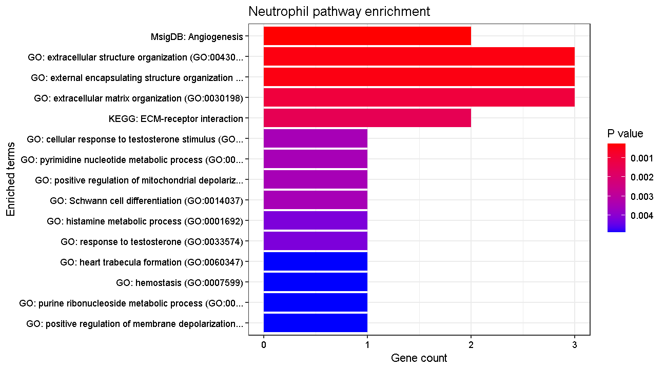
plot of chunk pway
OK, these results look appropriate for neutrophil biological function!
Session Info
sessionInfo()
R version 4.4.0 (2024-04-24 ucrt)
Platform: x86_64-w64-mingw32/x64
Running under: Windows 10 x64 (build 19045)

Matrix products: default


locale:
[1] LC_COLLATE=English_United States.utf8
[2] LC_CTYPE=English_United States.utf8
[3] LC_MONETARY=English_United States.utf8
[4] LC_NUMERIC=C
[5] LC_TIME=English_United States.utf8

time zone: America/New_York
tzcode source: internal

attached base packages:
[1] stats4    stats     graphics  grDevices utils     datasets  methods
[8] base

other attached packages:
 [1] enrichR_3.2                 DESeq2_1.44.0
 [3] SummarizedExperiment_1.34.0 Biobase_2.64.0
 [5] MatrixGenerics_1.16.0       matrixStats_1.4.1
 [7] GenomicRanges_1.56.2        GenomeInfoDb_1.40.1
 [9] IRanges_2.38.1              S4Vectors_0.42.1
[11] BiocGenerics_0.50.0         harmony_1.2.1
[13] Rcpp_1.0.13                 Seurat_5.1.0
[15] SeuratObject_5.0.2          sp_2.1-4
[17] lubridate_1.9.3             forcats_1.0.0
[19] stringr_1.5.1               dplyr_1.1.4
[21] purrr_1.0.2                 readr_2.1.5
[23] tidyr_1.3.1                 tibble_3.2.1
[25] ggplot2_3.5.1               tidyverse_2.0.0
[27] knitr_1.48

loaded via a namespace (and not attached):
  [1] RcppAnnoy_0.0.22        splines_4.4.0           later_1.3.2
  [4] polyclip_1.10-7         fastDummies_1.7.4       lifecycle_1.0.4
  [7] globals_0.16.3          lattice_0.22-6          vroom_1.6.5
 [10] MASS_7.3-61             magrittr_2.0.3          limma_3.60.4
 [13] plotly_4.10.4           httpuv_1.6.15           sctransform_0.4.1
 [16] spam_2.11-0             spatstat.sparse_3.1-0   reticulate_1.39.0
 [19] cowplot_1.1.3           pbapply_1.7-2           RColorBrewer_1.1-3
 [22] abind_1.4-8             zlibbioc_1.50.0         Rtsne_0.17
 [25] presto_1.0.0            WriteXLS_6.7.0          GenomeInfoDbData_1.2.12
 [28] ggrepel_0.9.6           irlba_2.3.5.1           listenv_0.9.1
 [31] spatstat.utils_3.1-0    goftest_1.2-3           RSpectra_0.16-2
 [34] spatstat.random_3.3-2   fitdistrplus_1.2-1      parallelly_1.38.0
 [37] leiden_0.4.3.1          codetools_0.2-20        DelayedArray_0.30.1
 [40] tidyselect_1.2.1        UCSC.utils_1.0.0        farver_2.1.2
 [43] spatstat.explore_3.3-2  jsonlite_1.8.9          progressr_0.14.0
 [46] ggridges_0.5.6          survival_3.7-0          tools_4.4.0
 [49] ica_1.0-3               glue_1.8.0              gridExtra_2.3
 [52] SparseArray_1.4.8       xfun_0.44               withr_3.0.1
 [55] fastmap_1.2.0           fansi_1.0.6             digest_0.6.35
 [58] timechange_0.3.0        R6_2.5.1                mime_0.12
 [61] colorspace_2.1-1        scattermore_1.2         tensor_1.5
 [64] spatstat.data_3.1-2     RhpcBLASctl_0.23-42     utf8_1.2.4
 [67] generics_0.1.3          data.table_1.16.2       httr_1.4.7
 [70] htmlwidgets_1.6.4       S4Arrays_1.4.1          uwot_0.2.2
 [73] pkgconfig_2.0.3         gtable_0.3.5            lmtest_0.9-40
 [76] XVector_0.44.0          htmltools_0.5.8.1       dotCall64_1.2
 [79] scales_1.3.0            png_0.1-8               spatstat.univar_3.0-1
 [82] rstudioapi_0.16.0       tzdb_0.4.0              reshape2_1.4.4
 [85] rjson_0.2.23            nlme_3.1-165            curl_5.2.3
 [88] zoo_1.8-12              KernSmooth_2.23-24      parallel_4.4.0
 [91] miniUI_0.1.1.1          vipor_0.4.7             ggrastr_1.0.2
 [94] pillar_1.9.0            grid_4.4.0              vctrs_0.6.5
 [97] RANN_2.6.2              promises_1.3.0          xtable_1.8-4
[100] cluster_2.1.6           beeswarm_0.4.0          evaluate_1.0.1
[103] cli_3.6.3               locfit_1.5-9.10         compiler_4.4.0
[106] rlang_1.1.4             crayon_1.5.3            future.apply_1.11.2
[109] labeling_0.4.3          plyr_1.8.9              ggbeeswarm_0.7.2
[112] stringi_1.8.4           viridisLite_0.4.2       deldir_2.0-4
[115] BiocParallel_1.38.0     munsell_0.5.1           lazyeval_0.2.2
[118] spatstat.geom_3.3-3     Matrix_1.7-0            RcppHNSW_0.6.0
[121] hms_1.1.3               patchwork_1.3.0         bit64_4.5.2
[124] future_1.34.0           statmod_1.5.0           shiny_1.9.1
[127] highr_0.11              ROCR_1.0-11             igraph_2.0.3
[130] bit_4.5.0
Key Points
Identifying cell types is a major objective in scRNA-Seq and can be present challenges that are unique to each dataset.
Statistically minded experimental design enables you to perform differential gene expression analyses that are likely to result in meaningful biological results.