Quality Control of scRNA-Seq Data
Overview
Teaching: 90 min
Exercises: 30 minQuestions
How do I determine if my single cell RNA-seq experiment data is high quality?
What are the common quality control metrics that I should check in my scRNA-seq data?
Objectives
Critically examine scRNA-seq data to identify potential technical issues.
Apply filters to remove cells that are largely poor quality/dead cells.
Understand the implications of different filtering steps on the data.
suppressPackageStartupMessages(library(tidyverse))
suppressPackageStartupMessages(library(Matrix))
suppressPackageStartupMessages(library(SingleCellExperiment))
suppressPackageStartupMessages(library(scds))
suppressPackageStartupMessages(library(Seurat))
data_dir <- '../data'
dir(data_dir)
 [1] "lesson03.Rdata"
 [2] "lesson03_challenge.Rdata"
 [3] "lesson04.rds"
 [4] "lesson05.Rdata"
 [5] "lesson05.rds"
 [6] "mouseStSt_exvivo"
 [7] "mouseStSt_exvivo.zip"
 [8] "mouseStSt_invivo"
 [9] "mouseStSt_invivo.zip"
[10] "regev_lab_cell_cycle_genes_mm.fixed.txt"
[11] "regev_lab_cell_cycle_genes_mm.fixed.txt_README"
Quality control in scRNA-seq
There are many technical reasons why cells produced by an scRNA-seq protocol might not be of high quality. The goal of the quality control steps are to assure that only single, live cells are included in the final data set. Ultimately some multiplets and poor quality cells will likely escape your detection and make it into your final dataset; however, these quality control steps aim to reduce the chance of this happening. Failure to undertake quality control is likely to adversely impact cell type identification, clustering, and interpretation of the data.
Some technical questions that you might ask include:
- Why is mitochondrial gene expression high in some cells?
- What is a unique molecular identifier (UMI), and why do we check numbers of UMI?
- What happens to make gene counts low in a cell?
Doublet detection
We will begin by discussing doublets. We have already discussed the concept of the doublet. Now we will try running one computational doublet-detection approach and track predictions of doublets.
We will use the scds method. scds contains two methods for predicting doublets. Method cxds is based on co-expression of gene pairs, while method bcds uses the full count information and a binary classification approach using in silico doublets. Method cxds_bcds_hybrid combines both approaches. We will use the combined approach. See Bais and Kostka 2020 for more details.
Because this doublet prediction method takes some time and is a bit memory-intensive, we will run it only on cells from one mouse. We will return to the doublet predictions later in this lesson.
cell_ids <- filter(metadata, sample == 'CS52') %>% pull(cell)
sce      <- SingleCellExperiment(list(counts = counts[, cell_ids]))
sce      <- cxds_bcds_hybrid(sce)
doublet_preds <- colData(sce)
            used   (Mb) gc trigger   (Mb)  max used   (Mb)
Ncells   8111953  433.3   14168290  756.7  11252398  601.0
Vcells 181810210 1387.2  436715070 3331.9 436711315 3331.9
High-level overview of quality control and filtering
First we will walk through some of the typical quantities one examines when conducting quality control of scRNA-Seq data.
Filtering Genes by Counts
As mentioned in an earlier lesson, the counts matrix is sparse and may contain rows (genes) or columns (cells) with low overall counts. In the case of genes, we likely wish to exclude genes with zeros counts in most cells. Let’s see how many genes have zeros counts across all cells. Note that the Matrix package has a special implementation of rowSums which works with sparse matrices.
gene_counts <- Matrix::rowSums(counts)
sum(gene_counts == 0)
[1] 7322
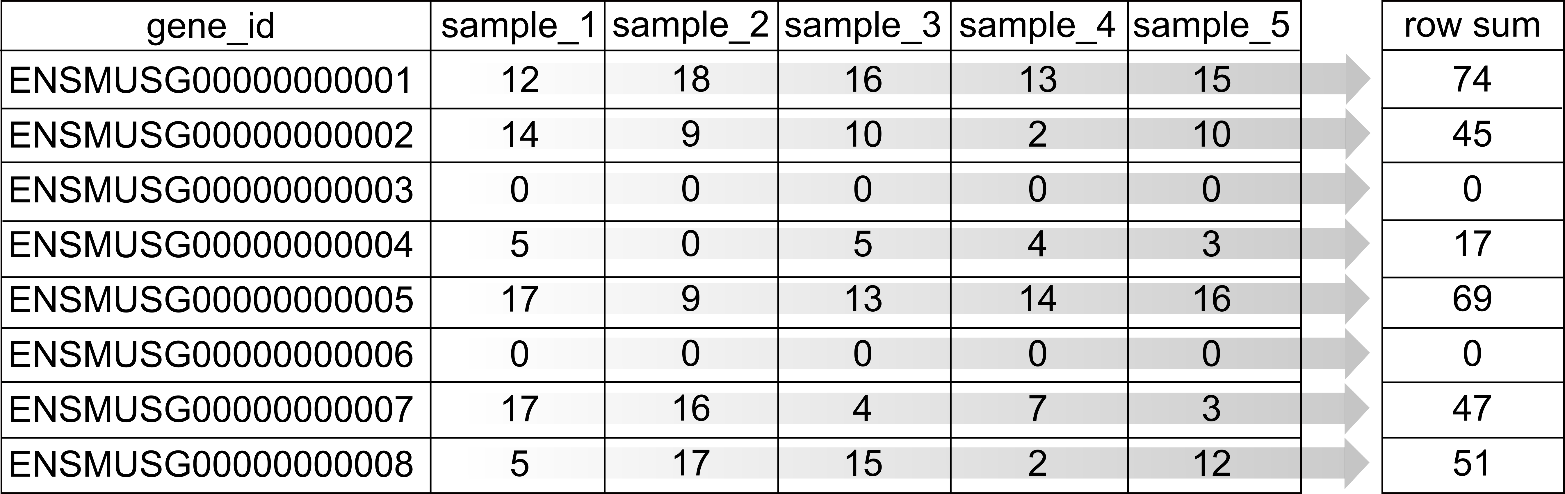
Of the 31053 genes, 7322 have zero counts across all cells. These genes do not inform us about the mean, variance, or covariance of any of the other genes and we will remove them before proceeding with further analysis.
counts <- counts[gene_counts > 0,]
This leaves 23731 genes in the counts matrix.
We could also set some other threshold for filtering genes. Perhaps we should
look at the number of genes that have different numbers of counts. We will use
a histogram to look at the distribution of overall gene counts. Note that, since
we just resized the counts matrix, we need to recalculate gene_counts.
We will count the number of cells in which each gene was detected. Because
counts is a sparse matrix, we have to be careful not to perform operations
that would convert the entire matrix into a non-sparse matrix. This might
happen if we wrote code like:
gene_counts <- rowSums(counts > 0)
The expression counts > 0 would create a logical matrix that takes up much
more memory than the sparse matrix. We might be tempted to try
rowSums(counts == 0), but this would also result in a non-sparse matrix
because most of the values would be TRUE. However, if we evaluate
rowSums(counts != 0), then most of the values would be FALSE, which can be
stored as 0 and so the matrix would still be sparse. The Matrix package has
an implementation of ‘rowSums()’ that is efficient, but you may have to specify
that you want to used the Matrix version of ‘rowSums()’ explicitly.
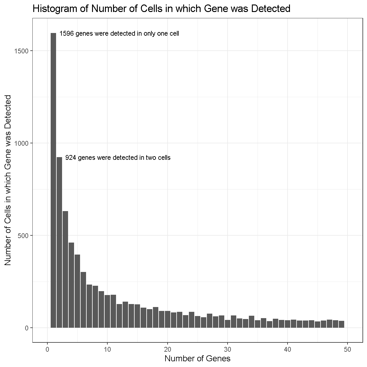
The number of cells in which each gene is detected spans several orders of magnitude and this makes it difficult to interpret the plot. Some genes are detected in all cells while others are detected in only one cell. Let’s zoom in on the part with lower gene counts.
gene_counts <- tibble(counts  = Matrix::rowSums(counts > 0))

gene_counts %>%
  dplyr::count(counts) %>%
  ggplot(aes(counts, n)) +
    geom_col() +
    labs(title = 'Histogram of Number of Cells in which Gene was Detected',
         x     = 'Number of Genes',
         y     = 'Number of Cells in which Gene was Detected') +
    lims(x = c(0, 50)) +
    theme_bw(base_size = 14) +
    annotate('text', x = 2, y = 1596, hjust = 0,
             label = str_c(sum(gene_counts == 1), ' genes were detected in only one cell')) +
    annotate('text', x = 3, y = 924, hjust = 0,
             label = str_c(sum(gene_counts == 2), ' genes were detected in two cells'))
Warning: Removed 9335 rows containing missing values or values outside the
scale range (`geom_col()`).
plot of chunk gene_count_hist_2
In the plot above, we can see that there are 1596 genes that were detected in only one cell, 924 genes detected in two cells, etc.
Making a decision to keep or remove a gene based on its expression being detected in a certain number of cells can be tricky. If you retain all genes, you may consume more computational resources and add noise to your analysis. If you discard too many genes, you may miss rare but important cell types.
Consider this example: You have a total of 10,000 cells in your scRNA-seq results. There is a rare cell population consisting of 100 cells that expresses 20 genes which are not expressed in any other cell type. If you only retain genes that are detected in more than 100 cells, you will miss this cell population.
Challenge 1
How would filtering genes too strictly affect your results? How would this affect your ability to discriminate between cell types?
Solution to Challenge 1
Filtering too strictly would make it more difficult to distinguish between cell types. The degree to which this problem affects your analyses depends on the degree of strictness of your filtering. Let’s take the situation to its logical extreme – what if we keep only genes expressed in at least 95% of cells. If we did this, we would end up with only 41 genes! By definition these genes will be highly expressed in all cell types, therefore eliminating our ability to clearly distinguish between cell types.
Challenge 2
What total count threshold would you choose to filter genes? Remember that there are 47,743 cells.
Solution to Challenge 2
This is a question that has a somewhat imprecise answer. Following from challenge one, we do not want to be too strict in our filtering. However, we do want to remove genes that will not provide much information about gene expression variability among the cells in our dataset. Our recommendation would be to filter genes expressed in < 5 cells, but one could reasonably justify a threshold between, say, 3 and 20 cells.
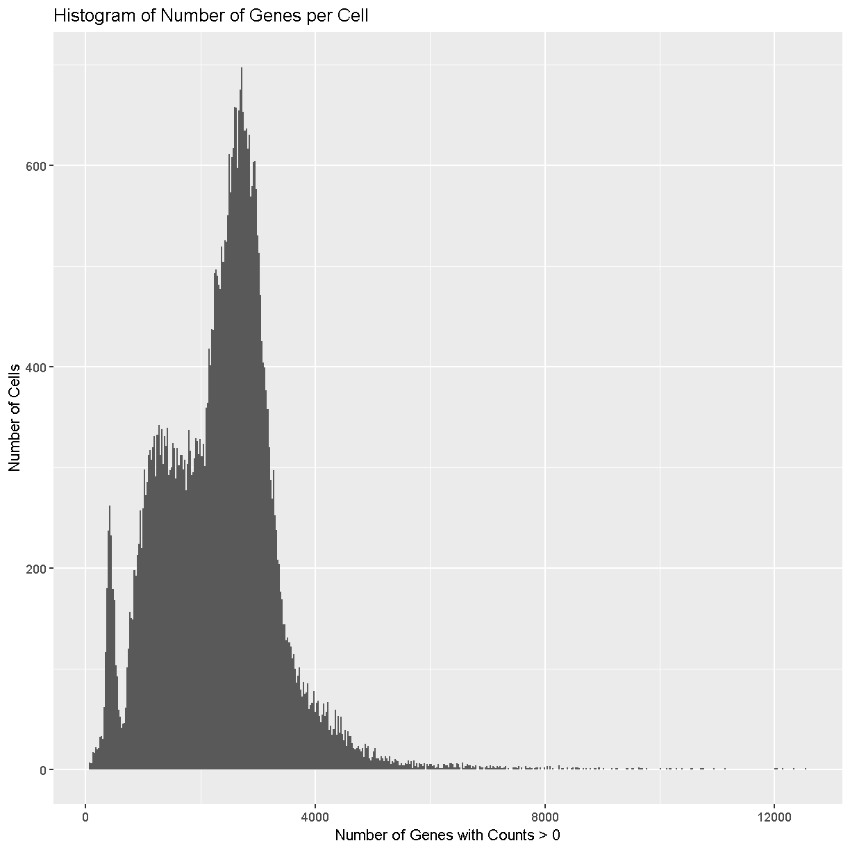
Filtering Cells by Counts
Next we will look at the number of genes expressed in each cell. If a cell lyses and leaks RNA,the total number of reads in a cell may be low, which leads to lower gene counts. Furthermore, each single cell suspension likely contains some amount of so-called “ambient” RNA from damaged/dead/dying cells. This ambient RNA comes along for the ride in every droplet. Therefore even droplets that do not contain cells (empty droplets) can have some reads mapping to transcripts that look like gene expression. Filtering out these kinds of cells is a quality control step that should improve your final results.
We will explicitly use the Matrix package’s implementation of ‘colSums()’.
tibble(counts  = Matrix::colSums(counts > 0)) %>%
  ggplot(aes(counts)) +
    geom_histogram(bins = 500) +
    labs(title = 'Histogram of Number of Genes per Cell',
         x     = 'Number of Genes with Counts > 0',
         y     = 'Number of Cells')
plot of chunk sum_cell_counts
Cells with way more genes expressed than the typical cell might be doublets/multiplets and should also be removed.
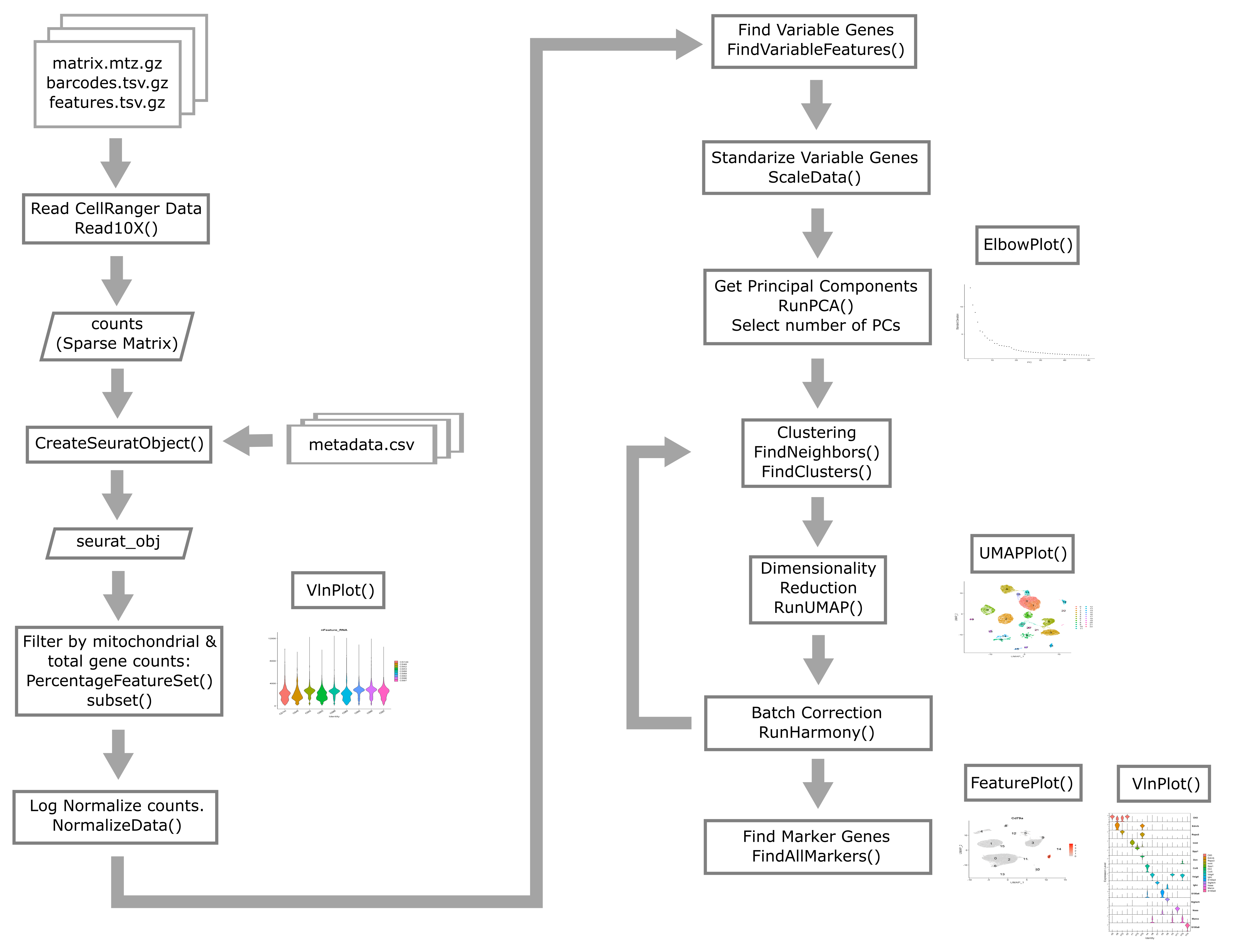
Creating the Seurat Object
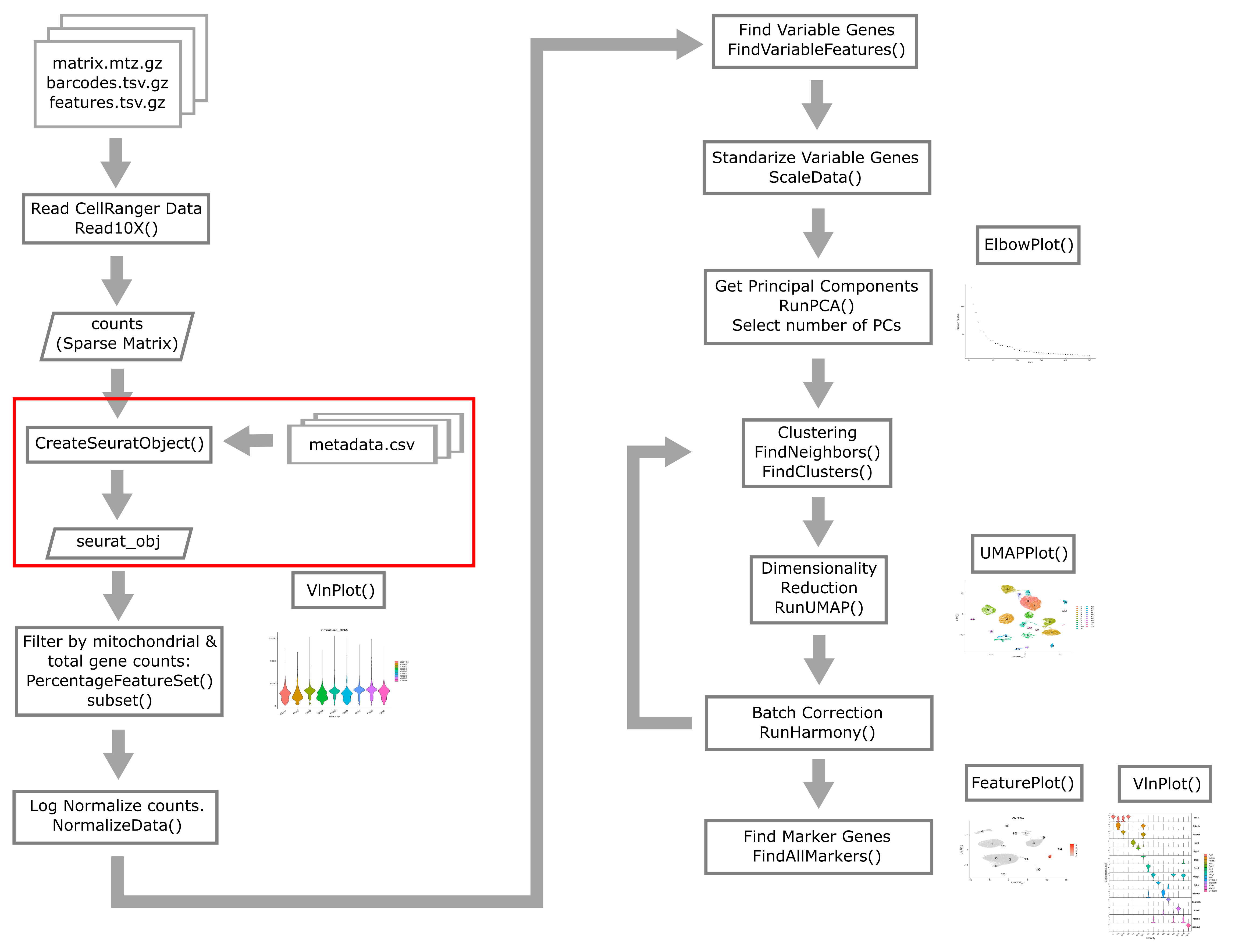
In order to use Seurat, we must take the sample metadata and gene counts and create a Seurat Object. This is a data structure which organizes the data and metadata and will store aspects of the analysis as we progress through the workshop.
Below, we will create a Seurat object for the liver data. We must first convert the cell metadata into a data.frame and place the barcodes in rownames. The we will pass the counts and metadata into the CreateSeuratObject function to create the Seurat object.
In the section above, we examined the counts across genes and cells and proposed filtering using thresholds. The CreateSeuratObject function contains two arguments, ‘min.cells’ and ‘min.features’, that allow us to filter the genes and cells by counts. Although we might use these arguments for convenience in a typical analysis, for this course we will look more closely at these quantities on a per-library basis to decide on our filtering thresholds. We will us the ‘min.cells’ argument to filter out genes that occur in less than 5 cells.
# set a seed for reproducibility in case any randomness used below
set.seed(1418)
metadata <- as.data.frame(metadata) %>%
              column_to_rownames('cell')
liver <- CreateSeuratObject(counts    = counts,
                            project   = 'liver: scRNA-Seq',
                            meta.data = metadata,
                            min.cells = 5)
We now have a Seurat object with 20,120 genes and 47,743 cells.
We will remove the counts object to save some memory because it is now stored inside of the Seurat object.
rm(counts)
gc()
            used   (Mb) gc trigger   (Mb)  max used   (Mb)
Ncells   8269380  441.7   14168290  756.7  12310063  657.5
Vcells 182530194 1392.6  596761865 4553.0 629553222 4803.2
Add on doublet predictions that we did earlier in this lesson.
liver <- AddMetaData(liver, as.data.frame(doublet_preds))
Let’s briefly look at the structure of the Seurat object. The counts are stored
as an assay, which we can query using the Assays() function.
Seurat::Assays(liver)
[1] "RNA"
The output of this function tells us that we have data in an “RNA assay. We can access this using the GetAssayData function.
tmp <- GetAssayData(object = liver, layer = 'counts')
tmp[1:5,1:5]
5 x 5 sparse Matrix of class "dgCMatrix"
       AAACGAATCCACTTCG-2 AAAGGTACAGGAAGTC-2 AACTTCTGTCATGGCC-2
Xkr4                    .                  .                  .
Rp1                     .                  .                  .
Sox17                   .                  .                  2
Mrpl15                  .                  .                  .
Lypla1                  .                  .                  2
       AATGGCTCAACGGTAG-2 ACACTGAAGTGCAGGT-2
Xkr4                    .                  .
Rp1                     .                  .
Sox17                   4                  .
Mrpl15                  1                  1
Lypla1                  1                  .
As you can see the data that we retrieved is a sparse matrix, just like the counts that we provided to the Seurat object.
What about the metadata? We can access the metadata as follows:
head(liver)
                         orig.ident nCount_RNA nFeature_RNA sample digest
AAACGAATCCACTTCG-2 liver: scRNA-Seq       8476         3264   CS48 inVivo
AAAGGTACAGGAAGTC-2 liver: scRNA-Seq       8150         3185   CS48 inVivo
AACTTCTGTCATGGCC-2 liver: scRNA-Seq       8139         3280   CS48 inVivo
AATGGCTCAACGGTAG-2 liver: scRNA-Seq      10083         3716   CS48 inVivo
ACACTGAAGTGCAGGT-2 liver: scRNA-Seq       9517         3543   CS48 inVivo
ACCACAACAGTCTCTC-2 liver: scRNA-Seq       7189         3064   CS48 inVivo
ACGATGTAGTGGTTCT-2 liver: scRNA-Seq       7437         3088   CS48 inVivo
ACGCACGCACTAACCA-2 liver: scRNA-Seq       8162         3277   CS48 inVivo
ACTGCAATCAACTCTT-2 liver: scRNA-Seq       7278         3144   CS48 inVivo
ACTGCAATCGTCACCT-2 liver: scRNA-Seq       9584         3511   CS48 inVivo
                   typeSample cxds_score bcds_score hybrid_score
AAACGAATCCACTTCG-2   scRnaSeq         NA         NA           NA
AAAGGTACAGGAAGTC-2   scRnaSeq         NA         NA           NA
AACTTCTGTCATGGCC-2   scRnaSeq         NA         NA           NA
AATGGCTCAACGGTAG-2   scRnaSeq         NA         NA           NA
ACACTGAAGTGCAGGT-2   scRnaSeq         NA         NA           NA
ACCACAACAGTCTCTC-2   scRnaSeq         NA         NA           NA
ACGATGTAGTGGTTCT-2   scRnaSeq         NA         NA           NA
ACGCACGCACTAACCA-2   scRnaSeq         NA         NA           NA
ACTGCAATCAACTCTT-2   scRnaSeq         NA         NA           NA
ACTGCAATCGTCACCT-2   scRnaSeq         NA         NA           NA
Notice that there are some columns that were not in our original metadata file; specifically the ‘nCount_RNA’ and ‘nFeature_RNA’ columns.
- nCount_RNA is the total counts for each cell.
- nFeature_RNA is the number of genes with counts > 0 in each cell.
These were calculated by Seurat when the Seurat object was created. We will use these later in the lesson.
Typical filters for cell quality
Here we briefly review these filters and decide what thresholds we will use for these data.
Filtering by Mitochondrial Gene Content
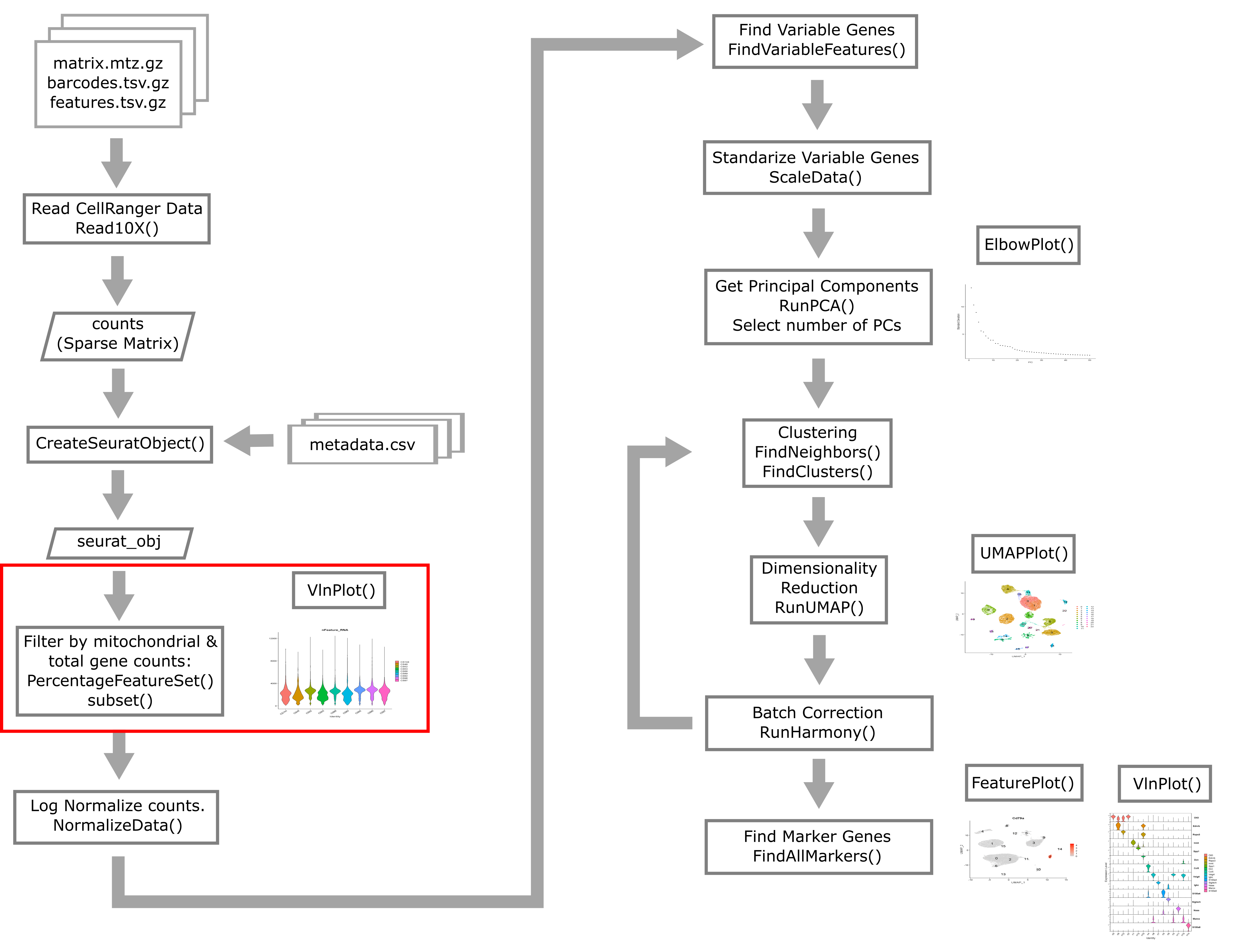
During apoptosis, the cell membrane may break and release transcripts into the surrounding media. However, the mitochondrial transcripts may remain inside of the mitochondria. This will lead to an apparent, but spurious, increase in mitochondrial gene expression. As a result, we use the percentage of mitochondrial-encoded reads to filter out cells that were not healthy during sample processing. See this link from 10X Genomics for additional information.
First we compute the percentage mitochondrial gene expression in each cell.
liver <- liver %>%
              PercentageFeatureSet(pattern = "^mt-", col.name = "percent.mt")
Different cell types may have different levels of mitochondrial RNA content. Therefore we must use our knowledge of the particular biological system that we are profiling in order to choose an appropriate threshold. If we are profiling single nuclei instead of single cells we might consider a very low threshold for MT content. If we are profiling a tissue where we anticipate broad variability in levels of mitochondrial RNA content between cell types, we might use a very lenient threshold to start and then return to filter out additional cells after we obtain tentative cell type labels that we have obtained by carrying out normalization and clustering. In this course we will filter only once
VlnPlot(liver, features = "percent.mt", group.by = 'sample')
Warning: Default search for "data" layer in "RNA" assay yielded no results;
utilizing "counts" layer instead.
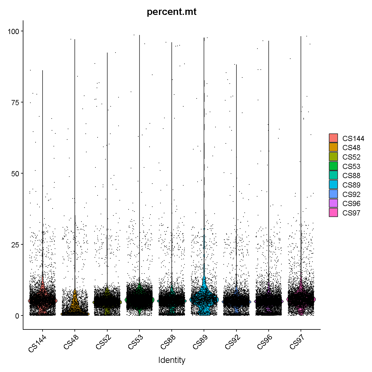
plot of chunk seurat_counts_plots
It is hard to see with so many dots! Let’s try another version where we just plot the violins:
VlnPlot(liver, features = "percent.mt", group.by = 'sample', pt.size = 0)
Warning: Default search for "data" layer in "RNA" assay yielded no results;
utilizing "counts" layer instead.
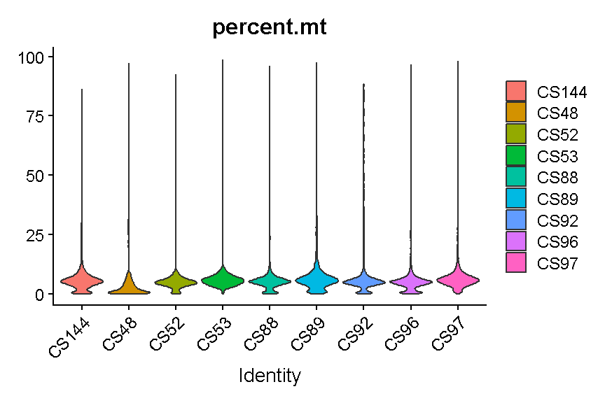
plot of chunk seurat_counts_plots2
Library “CS89” (and maybe CS144) have a “long tail” of cells with high mitochondrial gene expression. We may wish to monitor these libraries throughout QC and decide whether it has problems worth ditching the sample.
In most cases it would be ideal to determine separate filtering thresholds on each scRNA-Seq sample. This would account for the fact that the characteristics of each sample might vary (for many possible reasons) even if the same tissue is profiled. However, in this course we will see if we can find a single threshold that works decently well across all samples. As you can see, the samples we are examining do not look drastically different so this may not be such an unrealistic simplification.
We will use a threshold of 14% mitochondrial gene expression which will
remove the “long tail” of cells with high percent.mt values. We could
also perhaps justify going as low as 10% to be more conservative,
but we likely would not want to go down to 5%, which would
remove around half the cells.
# Don't run yet, we will filter based on several criteria below
#liver <- subset(liver, subset = percent.mt < 14)
Filtering Cells by Total Gene Counts
Let’s look at how many genes are expressed in each cell. Again we’ll split by the mouse ID so we can see if there are particular samples that are very different from the rest. Again we will show only the violins for clarity.
VlnPlot(liver, 'nFeature_RNA', group.by = 'sample', pt.size = 0)
Warning: Default search for "data" layer in "RNA" assay yielded no results;
utilizing "counts" layer instead.
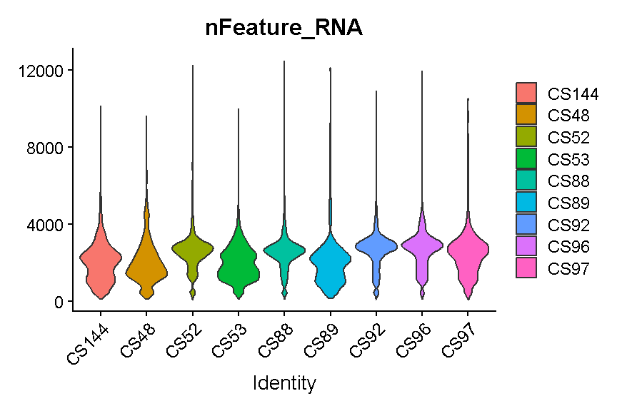
plot of chunk filter_gene_counts
Like with the mitochondrial expression percentage, we will strive to find a threshold that works reasonably well across all samples. For the number of genes expressed we will want to filter out both cells that express to few genes and cells that express too many genes. As noted above, damaged or dying cells may leak RNA, resulting in a low number of genes expressed, and we want to filter out these cells to ignore their “damaged” transcriptomes. On the other hand, cells with way more genes expressed than the typical cell might be doublets/multiplets and should also be removed.
It looks like filtering out cells that express less than 400 or greater than 5,000 genes is a reasonable compromise across our samples. (Note the log scale in this plot, which is necessary for seeing the violin densities at low numbers of genes expressed).
VlnPlot(liver, 'nFeature_RNA', group.by = 'sample', pt.size = 0) +
  scale_y_log10() +
  geom_hline(yintercept = 600) +
  geom_hline(yintercept = 5000)
Warning: Default search for "data" layer in "RNA" assay yielded no results;
utilizing "counts" layer instead.
Scale for y is already present.
Adding another scale for y, which will replace the existing scale.
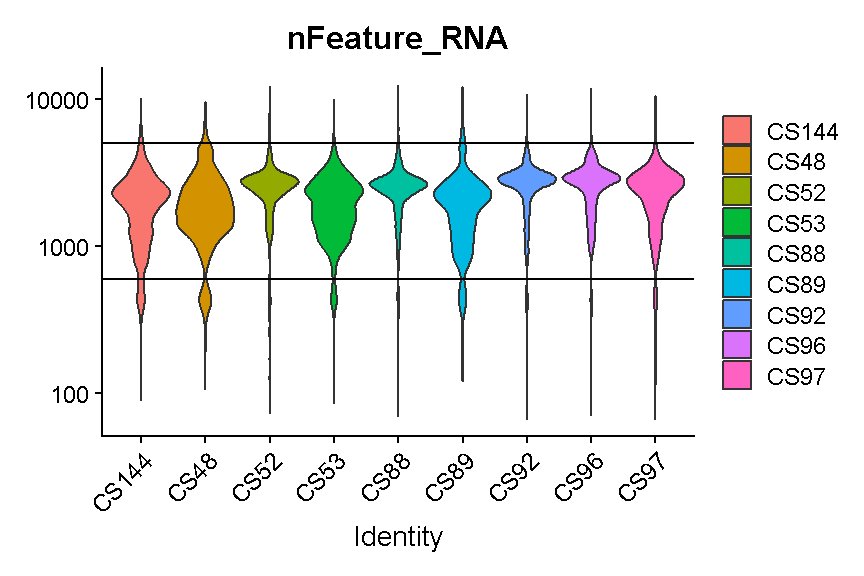
plot of chunk filter_gene_counts_5k
#liver <- subset(liver, nFeature_RNA > 600 & nFeature_RNA < 5000)
Filtering Cells by UMI
A UMI – unique molecular identifier – is like a molecular barcode for each RNA molecule in the cell. UMIs are short, distinct oligonucleotides attached during the initial preparation of cDNA from RNA. Therefore each UMI is unique to a single RNA molecule.
Why are UMI useful? The amount of RNA in a single cell is quite low (approximately 10-30pg according to this link). Thus single cell transcriptomics profiling usually includes a PCR amplification step. PCR amplification is fairly “noisy” because small stochastic sampling differences can propagate through exponential amplification. Using UMIs, we can throw out all copies of the molecule except one (the copies we throw out are called “PCR duplicates”).
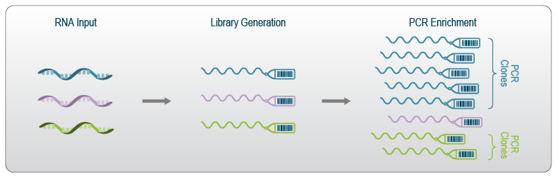
Several papers (e.g. Islam et al) have demonstrated that UMIs reduce amplification noise in single cell transcriptomics and thereby increase data fidelity. The only downside of UMIs is that they cause us to throw away a lot of our data (perhaps as high as 90% of our sequenced reads). Nevertheless, we don’t want those reads if they are not giving us new information about gene expression, so we tolerate this inefficiency.
CellRanger will automatically process your UMIs and the feature-barcode matrix it produces will be free from PCR duplicates. Thus, we can think of the number of UMIs as the sequencing depth of each cell.
Typically the number of genes and number of UMI are highly correlated and this is mostly the case in our liver dataset:
ggplot(liver@meta.data, aes(x = nCount_RNA, y = nFeature_RNA)) +
  geom_point() +
  theme_bw(base_size = 16) +
  xlab("nUMI") + ylab("nGenes") +
  scale_x_log10() + scale_y_log10()
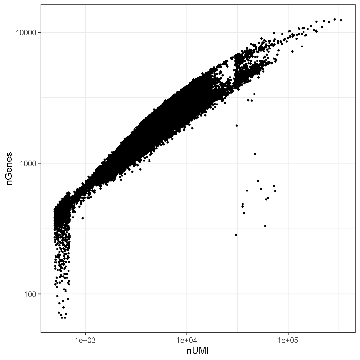
plot of chunk genes_umi
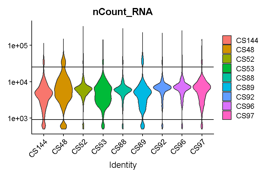
VlnPlot(liver, 'nCount_RNA', group.by = 'sample', pt.size = 0) +
  scale_y_log10() +
  geom_hline(yintercept = 900) +
  geom_hline(yintercept = 25000)
Warning: Default search for "data" layer in "RNA" assay yielded no results;
utilizing "counts" layer instead.
Scale for y is already present.
Adding another scale for y, which will replace the existing scale.
plot of chunk filter_umi
# Don't run yet, we will filter based on several criteria below
#liver <- subset(liver, nCount_RNA > 900 & nCount_RNA < 25000)
Again we try to select thresholds that remove most of the strongest outliers in all samples.
Challenge 2
List two technical issues that can lead to poor scRNA-seq data quality and which filters we use to detect each one.
Solution to Challenge 2
1 ). Cell membranes may rupture during the disassociation protocol, which is indicated by high mitochondrial gene expression because the mitochondrial transcripts are contained within the mitochondria, while other transcripts in the cytoplasm may leak out. Use the mitochondrial percentage filter to try to remove these cells.
2 ). Cells may be doublets of two different cell types. In this case they might express many more genes than either cell type alone. Use the “number of genes expressed” filter to try to remove these cells.
Doublet detection revisited
Let’s go back to our doublet predictions. How many of the cells that are going to be filtered out of our data were predicted to be doublets by scds?
liver$keep <- liver$percent.mt   < 14 &
              liver$nFeature_RNA > 600 &
              liver$nFeature_RNA < 5000 &
              liver$nCount_RNA   > 900 &
              liver$nCount_RNA   < 25000
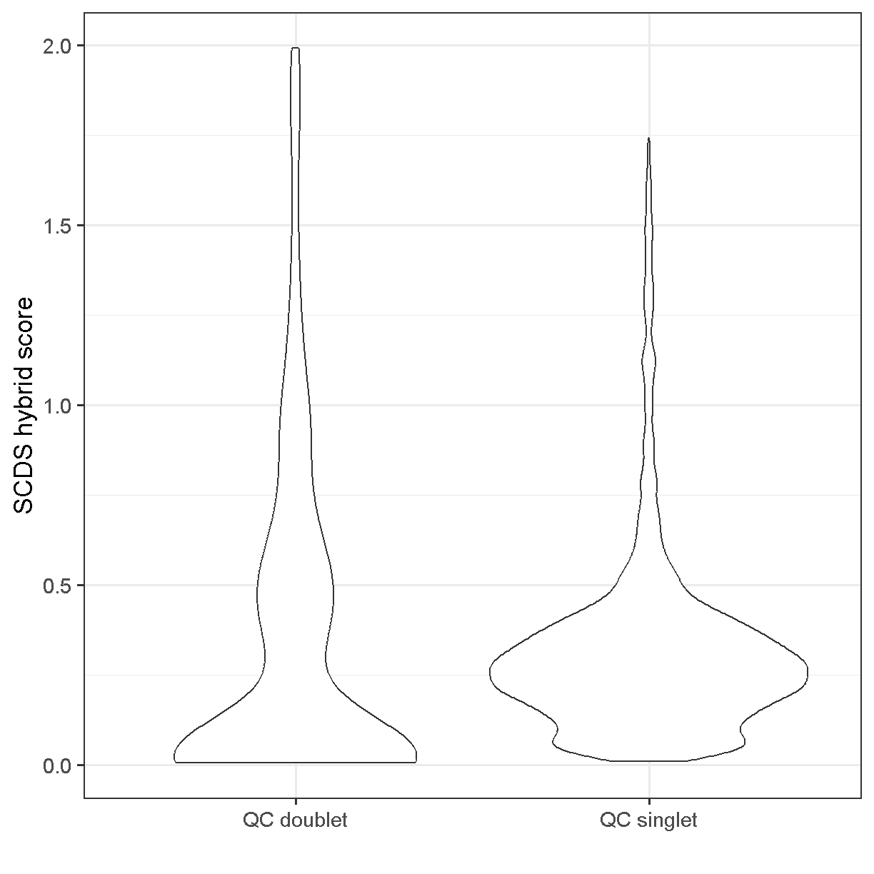
Using the scds hybrid_score method, the scores range between 0 and 2. Higher scores should be more likely to be doublets.
ggplot(mutate(liver[[]], class = ifelse(keep, 'QC singlet', 'QC doublet')),
  aes(x = class, y = hybrid_score)) +
  geom_violin() +
  theme_bw(base_size = 18) +
  xlab("") +
  ylab("SCDS hybrid score")
Warning: Removed 42388 rows containing non-finite outside the scale range
(`stat_ydensity()`).
plot of chunk doublet_plot
Somewhat unsatisfyingly, the scds hybrid scores aren’t wildly different between the cells we’ve used QC thresholds to call as doublets vs singlets. There does seem to be an enrichment of cells with score >0.75 among the QC doublets. If we had run scds doublet prediction on all cells we might compare results with no scds score filtering to those with an scds score cutoff of, say, 1.0. One characteristic of the presence of doublet cells is a cell cluster located between two large and well-defined clusters that expresses markers of both of them (don’t worry, we will learn how to cluster and visualize data soon). Returning to the scds doublet scores, we could cluster our cells with and without doublet score filtering, and see if we note any putative doublet clusters.
Subset based on %MT, number of genes, and number of UMI thresholds
liver <- subset(liver, subset = percent.mt   < 14 &
                                nFeature_RNA > 600 &
                                nFeature_RNA < 5000 &
                                nCount_RNA   > 900 &
                                nCount_RNA   < 25000)
Batch correction
We might want to correct for batch effects. This can be difficult to do because batch effects are complicated (in general), and may affect different cell types in different ways. Although correcting for batch effects is an important aspect of quality control, we will discuss this procedure in lesson 06 with some biological context.
Challenge 3
Delete the existing counts and metadata objects. Read in the ex-vivo data that you saved at the end of Lesson 03 (lesson03_challenge.Rdata) and create a Seurat object called ‘liver_2’. Look at the filtering quantities and decide whether you can use the same cell and feature filters that were used to create the Seurat object above.
Solution to Challenge 3
# Remove the existing counts and metadata.
rm(counts, metadata)
# Read in citeseq counts & metadata.
load(file = file.path(data_dir, 'lesson03_challenge.Rdata'))
# Create Seurat object.
metadata = as.data.frame(metadata) %>%
` column_to_rownames(‘cell’)liver_2 = CreateSeuratObject(count = counts, `
` project = ‘liver: ex-vivo’,meta.data = metadata)`
Challenge 4
Estimate the proportion of mitochondrial genes. Create plots of the proportion of features, cells, and mitochondrial genes. Filter the Seurat object by mitochondrial gene expression.
Solution to Challenge 4
liver_2 = liver_2 %>%` PercentageFeatureSet(pattern = “^mt-“, col.name = “percent.mt”)VlnPlot(liver_2, features = c(“nFeature_RNA”, “nCount_RNA”, “percent.mt”), ncol = 3)liver_2 = subset(liver_2, subset = percent.mt < 10)`
Session Info
sessionInfo()
R version 4.4.0 (2024-04-24 ucrt)
Platform: x86_64-w64-mingw32/x64
Running under: Windows 10 x64 (build 19045)

Matrix products: default


locale:
[1] LC_COLLATE=English_United States.utf8
[2] LC_CTYPE=English_United States.utf8
[3] LC_MONETARY=English_United States.utf8
[4] LC_NUMERIC=C
[5] LC_TIME=English_United States.utf8

time zone: America/New_York
tzcode source: internal

attached base packages:
[1] stats4    stats     graphics  grDevices utils     datasets  methods
[8] base

other attached packages:
 [1] Seurat_5.1.0                SeuratObject_5.0.2
 [3] sp_2.1-4                    scds_1.20.0
 [5] SingleCellExperiment_1.26.0 SummarizedExperiment_1.34.0
 [7] Biobase_2.64.0              GenomicRanges_1.56.2
 [9] GenomeInfoDb_1.40.1         IRanges_2.38.1
[11] S4Vectors_0.42.1            BiocGenerics_0.50.0
[13] MatrixGenerics_1.16.0       matrixStats_1.4.1
[15] Matrix_1.7-0                lubridate_1.9.3
[17] forcats_1.0.0               stringr_1.5.1
[19] dplyr_1.1.4                 purrr_1.0.2
[21] readr_2.1.5                 tidyr_1.3.1
[23] tibble_3.2.1                ggplot2_3.5.1
[25] tidyverse_2.0.0             knitr_1.48

loaded via a namespace (and not attached):
  [1] RColorBrewer_1.1-3      rstudioapi_0.16.0       jsonlite_1.8.9
  [4] magrittr_2.0.3          ggbeeswarm_0.7.2        spatstat.utils_3.1-0
  [7] farver_2.1.2            zlibbioc_1.50.0         vctrs_0.6.5
 [10] ROCR_1.0-11             spatstat.explore_3.3-2  htmltools_0.5.8.1
 [13] S4Arrays_1.4.1          xgboost_1.7.8.1         SparseArray_1.4.8
 [16] pROC_1.18.5             sctransform_0.4.1       parallelly_1.38.0
 [19] KernSmooth_2.23-24      htmlwidgets_1.6.4       ica_1.0-3
 [22] plyr_1.8.9              plotly_4.10.4           zoo_1.8-12
 [25] igraph_2.0.3            mime_0.12               lifecycle_1.0.4
 [28] pkgconfig_2.0.3         R6_2.5.1                fastmap_1.2.0
 [31] GenomeInfoDbData_1.2.12 fitdistrplus_1.2-1      future_1.34.0
 [34] shiny_1.9.1             digest_0.6.35           colorspace_2.1-1
 [37] patchwork_1.3.0         tensor_1.5              RSpectra_0.16-2
 [40] irlba_2.3.5.1           labeling_0.4.3          progressr_0.14.0
 [43] spatstat.sparse_3.1-0   fansi_1.0.6             timechange_0.3.0
 [46] polyclip_1.10-7         httr_1.4.7              abind_1.4-8
 [49] compiler_4.4.0          withr_3.0.1             fastDummies_1.7.4
 [52] highr_0.11              MASS_7.3-61             DelayedArray_0.30.1
 [55] tools_4.4.0             vipor_0.4.7             lmtest_0.9-40
 [58] beeswarm_0.4.0          httpuv_1.6.15           future.apply_1.11.2
 [61] goftest_1.2-3           glue_1.8.0              nlme_3.1-165
 [64] promises_1.3.0          grid_4.4.0              Rtsne_0.17
 [67] cluster_2.1.6           reshape2_1.4.4          generics_0.1.3
 [70] spatstat.data_3.1-2     gtable_0.3.5            tzdb_0.4.0
 [73] data.table_1.16.2       hms_1.1.3               utf8_1.2.4
 [76] XVector_0.44.0          spatstat.geom_3.3-3     RcppAnnoy_0.0.22
 [79] ggrepel_0.9.6           RANN_2.6.2              pillar_1.9.0
 [82] spam_2.11-0             RcppHNSW_0.6.0          later_1.3.2
 [85] splines_4.4.0           lattice_0.22-6          deldir_2.0-4
 [88] survival_3.7-0          tidyselect_1.2.1        miniUI_0.1.1.1
 [91] pbapply_1.7-2           gridExtra_2.3           scattermore_1.2
 [94] xfun_0.44               stringi_1.8.4           UCSC.utils_1.0.0
 [97] lazyeval_0.2.2          evaluate_1.0.1          codetools_0.2-20
[100] cli_3.6.3               uwot_0.2.2              xtable_1.8-4
[103] reticulate_1.39.0       munsell_0.5.1           Rcpp_1.0.13
[106] spatstat.random_3.3-2   globals_0.16.3          png_0.1-8
[109] ggrastr_1.0.2           spatstat.univar_3.0-1   parallel_4.4.0
[112] dotCall64_1.2           listenv_0.9.1           viridisLite_0.4.2
[115] scales_1.3.0            ggridges_0.5.6          leiden_0.4.3.1
[118] crayon_1.5.3            rlang_1.1.4             cowplot_1.1.3
Key Points
It is essential to filter based on criteria including mitochondrial gene expression and number of genes expressed in a cell.
Determining your filtering thresholds should be done separately for each experiment, and these values can vary dramatically in different settings.